Introduction to Principal Components Analysis

PCA (Principal Components Analysis) is a popular statistical method to reduce dimensions when the dimension of a dataset is huge, especially, when $n \geq m$ in $m \times n$ matrix or dataset.

Before digging into PCA, I start with some basic of linear algebra.

1. Numerator and Denominator Layout in Matrix Differentiation

In matrix differentiation, there are two notational convention to express the derivative of a vector with respect to a vector, that is $\frac{\partial y}{\partial x}$, which are “Numerator Layout” and “Denominator Layout”.

It doesn’t matter which way you would like to use, but make sure you stick with a notational convention if you start with a particular convention.

Let $x$ be a $n \times 1$ vector, $y$ be a $m \times 1$ vector.

Then, for $\frac{\partial y}{\partial x}$,

Numerator Layout: $m \times n$ matrix as following;

Denominator Layout: $n \times m$ matrix as following;

The different kinds of two notational convention can be found from Wiki

Most of books or papers don’t state which convention they use, but the Denominator Layout is mostly used in many papers or software. This article is going to use Denominator Layout in this article.

2. Variance-Covariance Matrix

Variance-Covariance Matrix, called just Covariance Matrix, of a matrix $X$ can be expressed in two ways as following;

$$S = \frac{1}{n-1} XX^T \tag{1}$$

or

$$S = \frac{1}{n-1} X^{T}X \tag{2}$$

where $X$ is the $m \times n$ matrix.

I will make the data be centered by subtracting the mean of the data for later convenience.

The (1) equation will give you the covariance matrix by row vectors as following;

$$S_{n \times n} = \frac{1}{n-1} X_{n \times 1} X_{1 \times n}^T = \frac{1}{n-1} \sum_{i=1}^{n} (x_i - \mu)(x_i - \mu)^T \tag{3}$$

where $\mu$ is the row mean vector and $S$ will be the $n \times n$ square matrix.

The (2) equation will give you the covariance matrix by column vectors as following;

$$S_{m \times m} = \frac{1}{n-1} X_{m \times 1}^{T}X_{1 \times m} = \frac{1}{n-1} \sum_{i=1}^{m} (x_i - \mu)^{T}(x_i - \mu) \tag{4}$$

where $\mu$ is the column mean vector and $S$ will be the $m \times m$ square matrix.

Example

Let $X$ be $2 \times 3$ matrix as the following;

$$X = \begin{bmatrix} 1 & 2 & 3 \\ 4 & 5 & 6 \end{bmatrix}$$

Then, for (1) equation,

The row vectors will be $3 \times 1$ vector as following;

$X_1 = \begin{bmatrix} 1 \\ 2 \\ 3 \end{bmatrix}$ and $X_2 = \begin{bmatrix} 4 \\ 5 \\ 6 \end{bmatrix}$.

Then, the covariance matrix will be

$$S_{3 \times 3} = \frac{1}{n-1} X_{3 \times 1} X_{1 \times 3}^{T}$$.

For (2) equation,

The column vectors will be $1 \times 2$ vectors as following;

$X_1 = \begin{bmatrix} 1 & 4 \end{bmatrix}$, $X_2 = \begin{bmatrix} 2 & 5 \end{bmatrix}$, $X_3 = \begin{bmatrix} 3 & 6 \end{bmatrix}$.

Then, the covariance matrix will be

$$S_{2 \times 2} = \frac{1}{n-1} X_{2 \times 1}^{T} X_{1 \times 2}$$

In this paper, we will need the (2) covariance matrix since mostly columns are the predictors, and covariance matrix is calculated by the columns.

3. Intuition on Eigenvalues and Eigenvectors

Formal Definition of Eigenvalues and Eigenvectors:

Let A be $n \times n$ a sqaure matrix, then $v$ and $\lambda$ is the Eigenvector and the Eigenvalue of $A$, respectively, if

$$Av = \lambda v \tag{5}$$

where $v$ is a non-zero vector and $\lambda$ can be any scalar.

Geometrical meaning of Eigenvectors and Eigenvalues would be..

From Wiki,

Eigenvectors can be seen the scaled direction vectors in the difrection of the particular vector; therefore, the direction of the vector is preserved, but we are just scaling the lengths.
Eigenvalue can be seen the factor by which it is stretched.

For equation (5), it is equivalent to the following;

$$(A - \lambda I)v = 0$$

where $I$ is the $n \times n$ identity matrix, and $0$ is the zero vector.

Also, if the $(A - \lambda I)$ is invertible, then $v$ can be zero-vector; therefore, in order to have a non-zero vector, $v$, the $(A - \lambda I)$ must be not invertible. It leads the determinant of $(A - \lambda I)$ must be zero as the following;

$$det(A - \lambda I) = 0$$

4. Eigendecomposition or Spectral Decomposition

Let $A$ be $n \times n$ a sqaure matrix with its rank is $n$, $rank(A) = n$, which is equivalent to have the number of linearly independent of columns or rows.

Then, $A$ can be factorized as

$$A_{n \times n} = Q_{n \times n} \Lambda_{n \times n} Q_{n \times n}^{-1}$$

where $Q$ is the $n \times n$ square matrix that the $i$th column is the eigenvector of A, and the $\Lambda$ is the diagonal matrix that the diagonal elements are the eigenvalues of A, $\Lambda_{ii} = \lambda_i$.

If the $Q$ is orthogonal matrix, then $A$ is equivalent to the following;

$$A = Q \Lambda Q^{-1} = Q \Lambda Q^T \tag{6}$$

5. SVD (Singular Value Decomposition)

Let $A$ be $m \times n$ a rectangular matrix, then $A$ can be factorized as,

$$A_{m \times n} = U_{m \times m} \Sigma_{m \times n} V_{n \times n}^{T}$$

where $U$ and $V$ is orthonormal square matrix, which means $U^{T}U = V^{T}V = I$, and $\Sigma$ is the diagonal matrix.

Then, the square matrix,

$$A_{m \times n}A_{n \times m}^{T} = (U \Sigma V^T) (U \Sigma V^T)^T \\ = (U \Sigma V^T) (V \Sigma^{T} U^{T}) \\ = U(\Sigma \Sigma^{T}) U^{T} \tag{7}$$

which gives us $U$ is the eigenvector of $AA^T$ by the definition of Eigendecomposition and the fact that we assume that $U$ is the orthonormal matrix, and $U$ is called left-singular vector.

$$A_{n \times m}^{T}A_{m \times n} = (U \Sigma V^T)^{T} (U \Sigma V^T) \\ = (V \Sigma^{T} U^{T}) (U \Sigma V^T) \\ = V (\Sigma^{T} \Sigma) V^{T} \tag{8}$$

which gives us $V$ is the eigenvector of $A^{T}A$ by the definition of Eigendecomposition and the fact that we assume that $V$ is the orthonormal matrix, and $V$ is called right-singular vector.

Also, $\Sigma \Sigma^{T} = \Sigma^{T} \Sigma$ is the diagonal matrix that the diagonal elements are the eigenvalues.

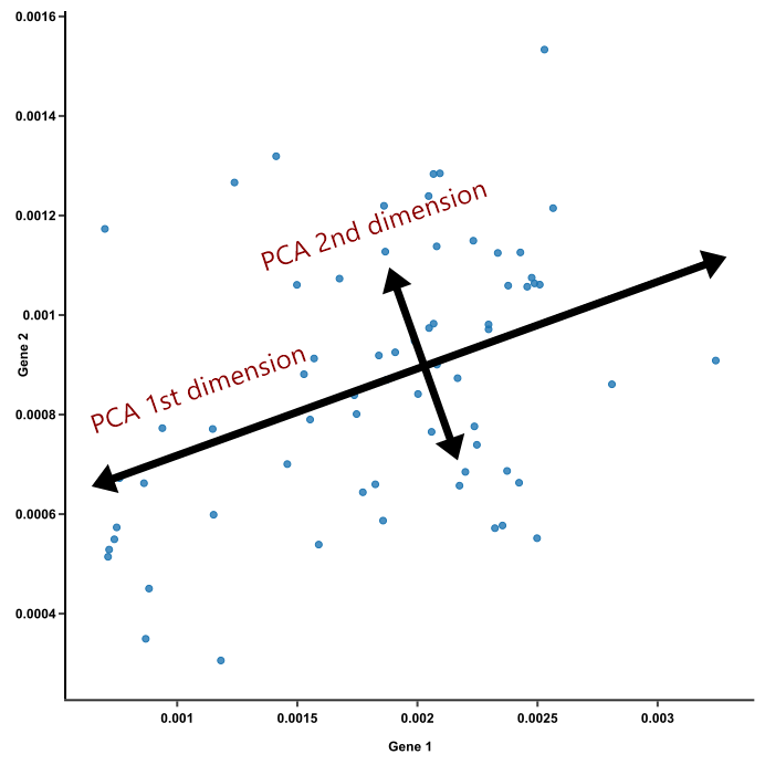
6. PCA (Principal Components)

The goal of the PCA is to identify the most meaningful basis to re-express a dataset.

Let $X$ be $m \times n$ matrix, $Y$ be another $m \times n$ matrix related by a linear transformation $P_{n \times n}$.

Then,

$$Y = XP \\ = \begin{bmatrix} x_{11} & \dots & x_{1n} \\ \vdots & \ddots \\ x_{m1} & \dots & x_{mn} \end{bmatrix} \begin{bmatrix} p_{11} & \dots & p_{1n} \\ \vdots & \ddots \\ p_{n1} & \dots & p_{nn} \end{bmatrix}$$

which gives us the dot product of $X$ and $P$.

The dot product can be interpreted as a linear transformation or projecting $X$ onto another basis by $P$.

In this case, let’s see the covariance matrix of $Y$. Notice that the covariance matrix of $Y$ or the covariance matrix of $X$ are centered as stated above (3) or (4).

$$C_{Y} = \frac{1}{n-1} Y^{T}Y \\ = \frac{1}{n-1} (XP)^{T}(XP) \\ = \frac{1}{n-1}(P^{T}X^{T}XP) \\ = P^{T}C_{X} P$$

If we prove that the matrix $P$ is orthonormal matrix, then we can see

$$C_{Y} = P^{T}C_{X} P = P^{-1}C_{X} P$$

by (6)

and hence, it implies that $P$ is the eigenvector matrix of covariance matrix of $X$.

1. First Approach to prove $P$ is orthonormal.

We know that $C_{Y}$ is the symmetric matrix since it is the covariance matrix of $Y$,

then, $C_{Y} = C_{Y}^{T}$ is true.

Let assume that $C_{Y} = P^{-1} C_{X} P$ by definition of Eigendecomposition.

$$C_{Y}^{T} = (P^{-1} C_{X} P)^{T} = (C_{X})^{T} (P^{-1})^{T} \\ = C_{Y} $$

Therefore,

$$P^{T} (C_{X})^{T} (P^{-1})^{T} = P^{T}C_{X} P$$

We know that $C_X = C_{X}^{T}$ since the covariance matrix of $X$ is symmetric matrix.

Finally,

$$P^{T} C_{X} (P^{-1})^{T} = P^{T}C_{X} P \\ (P^{-1})^{T} = P$$

Now, we can see the $P$ is orthonormal matrix.

This proof implies that we can get the $P$ from SVD by calculating $V$.

The covariance matrix of $X$ is..

$$C_X = \frac{1}{n-1} X^{T}X$$

By (8) in SVD, $X^{T}X$ is..

$$X^{T}X = V (\Sigma_{X}^{T} \Sigma_{X}) V^{T}$$

Therefore,

$$V^{T} = P$$

2. Second Approach to prove $P$ is orthonormal (this proof was provided by a member of my study group)

We have

$$Y = XP$$

where $Y$ is the projected values for $X$ by linear tranformation of $P$.

Suppose we have $U$ as the following;

$$YU = X_{recovered}$$

where $X_{recovered}$ is the re-proejcted values onto original values from the basis where the dataset are projected onto.

Then,

$$XPU = X_{recovered}$$

Therefore,

$$PU = I \tag{9}$$

Let $x$ is column vectors from $X$, and $\hat{x}$ is column vectors from $Y$.

$$x_{n \times 1} \in X_{m \times n}, \hat{x_{n \times 1}} \in Y_{m \times n}$$

The loss function of PCA is

$$\arg\min_{\hat{x}} ||x_{n \times 1} - U_{n \times n}\hat{x_{n \times 1}}||$$

To optimize, we differentiate the equation with respect to $\hat{x}$.

$$\frac{\partial}{\partial \hat{x}} ||x - U\hat{x}|| \\ = \frac{\partial}{\partial \hat{x}} (x-U\hat{x})^{T}(x-U\hat{x}) \\ = \frac{\partial}{\partial \hat{x}} (x^T - \hat{x}^{T}U^{T})(x-U\hat{x}) \\ = \frac{\partial}{\partial \hat{x}} (x^{T}x - \hat{x}^{T}U^{T}x - x^{T}U\hat{x} + \hat{x}^{T}\hat{x}) $$

Here, $\hat{x}^{T}U^{T}x = x^{T}U\hat{x}$ since they are scalar value.

$$= \frac{\partial}{\partial \hat{x}} (x^{T}x - 2x^{T}U\hat{x} + \hat{x}^{T}\hat{x}) \\ = 0 - 2U^{T}x + 2\hat{x} \tag{10}$$

By denominator layout as explained above,

$$\frac{\partial}{\partial \hat{x}} \hat{x}^{T}\hat{x} = 2\hat{x}$$

$$\frac{\partial}{\partial \hat{x}} x^{T}U\hat{x} = (x^{T}U)^{T} = U^{T}x$$

Set the (10) equation as zero,

$$ - 2U^{T}x + 2\hat{x} = 0 \\ \hat{x} = U^{T}x$$

Therefore, $\hat{x} = Px$ from the first assumption, and $P = U^{T}$.

From (9) equation,

$$PU = PP^T = I \\ P^{-1} = P^T$$

We proved that $P$ is the orthonormal matrix.

As a result,

1. $P$ is the Principal Components that allows us to get the most meaningful basis to re-express our dataset by linear transforming our dataset.
2. $P$ is the eigenvector matrix of the covariance matrix of our dataset for the column vectors (predictors)
3. $P$ is the transpose of right-singular vector, which is the $V^T$ in $U \Sigma V^T$, from Singular Value Decomposition.

Reference:
A Tutorial on Principal Component Analysis
Singular Value Decomposition and Principal Component Analysis
HOW ARE PRINCIPAL COMPONENT ANALYSIS AND SINGULAR VALUE DECOMPOSITION RELATED?
Matrix Differentiation
Eigenvalues and eigenvectors
Eigendecompositoin of a matrix
Matrix Calculus
Understanding Principal Component Analysis Once And For All

Introduction to the Cholesky Decomposition.

Cholesky Decomposition is used for its superior efficiency in linear calculation, such as affine function, $Ax = b$. Among many applications of Cholesky Decomposition, I will discuss about how the multivariate normal random numbers are generated with Cholesky Decomposition.

$\large{Definition}$:

Every positive definite matrix $A \in \mathcal{R}^{n \times n}$,

The Cholesky Decomposition is a form of

$$A = LL^{T}$$

where $L$ is the lower triangular matrix with real and positive diagonal elements. $L$ is called Cholesky factor of $A$ and it can be interpreted as the square root of a positive definite matrix.

$\large{Algorithm}$:

This algorithm is used in this link, and there are many apporaches to decompose a matrix with Cholesky Decomposition.

1. Compute $L_{1} = \sqrt{a_{11}}$
2. For $k = 2, … ,n$, find $L_{k-1}l_{k} = a_{k} for l_{k}$
3. $l_{kk} = \sqrt{a_{kk}-l_{k}^{T}l_{k}}$
4. $L_{k} = \begin{bmatrix} L_{k-1} & 0 \\ l_{k}^{T} & l_{kk} \end{bmatrix}$

then $L_{k}$ is the lower triangular matrix of Cholesky Decomposition.

Other approaches;

• Cholesky Decomposition
• link

$\large{Generating}$ $\large{Multivariate}$ $\large{Normal}$ $\large{Random}$ $\large{Number}$ $\large{with}$ $\large{Cholesky}$ $\large{Decomposition}$

If we have $X$ that follows Normal Distribution,

then

$$X \sim \mathcal{N}(\mu, \Sigma)$$

Let $Z$ follows standard normal distribution with mean 0 and variance 1.

Then,

$$Z \sim \mathcal{N}(0,I)$$

Then, we can express the $X$ with $Z$ as the following;

$$X = A+BZ$$

then $X$ will follow normal distribution as the following;

$$X \sim \mathcal{N}(A,BB’)$$

Here, $\mu$ is the $A$, and $\Sigma$ is the $BB’$. The $B$ is the lower triangular matrix of the decomposed $X$, which is the Cholesky factor.

Therefore, If we have a Cholesky factor, $B$, of covariance matrix of $X$, then the product of $B$ and standard normal random number matrix will generate the multivariate normal random number associated with the mean $\mu$ and covariance $\Sigma$ of $X$.

Reference:

Cholesky Decomposition
Cholesky Factorization
Cholesky Decomposition with R example
link
Bivariate Normal Distribution

Brief introduction to Schur Complement.

This is just a brief introduction of the properties of Schur Complement. Schur Complement has many applications in numerical analysis, such as optimization, machine learning algorithms, or probability and matrix theories.

Let’s begin with the definition of the Schur Complement.

$\large{Definition}$:

The Schur Complement of a black matrix is defined as;

Let $M$ be $n \times n$ matrix

$$M = \begin{bmatrix} A & B \\ C & D \end{bmatrix}$$

Then, the Schur Complement of the block $D$ of the matrix $M$ is

$$M/D := A - BD^{-1}C$$

if $D$ is invertible.

The Schur Complement of the block $A$ of the matrix $M$ is then,

$$M/A := D - CA^{-1}B$$

if $A$ is invertible.

$$\large{Properties}$$

• Linear system

Let
$A$ is a $p \times p$ matrix,
$D$ is a $q \times q$ matrix, with $n = p + q$
So, $B$ is a $p \times q$ matrix.

Let $M$ be defined as,

$$M = \begin{bmatrix} A & B \\ B^{T} & D \end{bmatrix}$$

Suppose we have a linear system as,

$$Ax + By = c \\ B^{T}x + Dy = d$$

Then,

$$\begin{bmatrix} A & B \\ B^{T} & D \end{bmatrix} \begin{bmatrix} x \\ y \end{bmatrix} = \begin{bmatrix} c \\ d \end{bmatrix}$$

Assuming $D$ is invertible,

then we have $y$ as

$$y = D^{-1}(d - B^{T}x)$$

Then, from the equation,

$$Ax + By = c \\ Ax + B(D^{-1}(d - B^{T}x)) = c$$

Then, we see that is,

$$(A - BD^{-1}B^{T})x = c - BD^{-1}d$$

Here, the $A - BD^{-1}B^{T}$ is the Schur Complement of a block $D$ of matrix $M$.

It follows,

$$x = (A-BD^{-1}B^{T})^{-1}(c-BD^{-1}d) \\ y = D^{-1}(d-B^{T}(A-BD^{-1}B^{T})^{-1}(c-BD^{-1}d))$$

And,

$$x = (A-BD^{-1}B^{T})^{-1}c - (A-BD^{-1}B^{T})^{-1}BD^{-1}d \\ y = -D^{-1}B^{T}(A-BD^{-1}B^{T})^{-1}c + (D^{-1}+D^{-1}B^{T}(A-BD^{-1}B^{T})^{-1}BD^{-1})d$$

The $x$ and $y$ are formed as linear functions associated with $c$ and $d$,

and it can be a formula for an inverse of $M$ in terms of the Schur Complement of $D$ in $M$.

$$\begin{bmatrix} A & B \\ B^{T} & D \end{bmatrix} ^{-1} = \begin{bmatrix} (A-BD^{-1}B^{T})^{-1} & -(A-BD^{-1}B^{T})^{-1}BD^{-1} \\ -D^{-1}B^{T}(A-BD^{-1}B^{T})^{-1} & D^{-1}+D^{-1}B^{T}(A-BD^{-1}B^{T})^{-1}BD^{-1} \end{bmatrix}$$

This can be written as,

$$\begin{bmatrix} A & B \\ B^{T} & D \end{bmatrix} ^{-1} = \begin{bmatrix} (A-BD^{-1}B^{T})^{-1} & 0 \\ -D^{-1}B^{T}(A-BD^{-1}B^{T})^{-1} & D^{-1} \end{bmatrix} \begin{bmatrix} I & -BD^{-1} \\ 0 & I \end{bmatrix}$$

Eventually,

$$\begin{bmatrix} A & B \\ B^{T} & D \end{bmatrix} ^{-1} = \begin{bmatrix} I & 0 \\ -D^{-1}B^{T} & I \end{bmatrix} \begin{bmatrix} (A-BD^{-1}B^{T})^{-1} & 0 \\ 0 & D^{-1} \end{bmatrix} \begin{bmatrix} I & -BD^{-1} \\ 0 & I \end{bmatrix}$$

If we take inverse on both sides,

$$\begin{bmatrix} A & B \\ B^{T} & D \end{bmatrix} = \begin{bmatrix} I & BD^{-1} \\ 0 & I \end{bmatrix} \begin{bmatrix} A-BD^{-1}B^{T} & 0 \\ 0 & D \end{bmatrix} \begin{bmatrix} I & 0 \\ D^{-1}B^{T} & I \end{bmatrix}$$

$$= \begin{bmatrix} I & BD^{-1} \\ 0 & I \end{bmatrix} \begin{bmatrix} A-BD^{-1}B^{T} & 0 \\ 0 & D \end{bmatrix} \begin{bmatrix} I & BD^{-1} \\ 0 & I \end{bmatrix} ^{T}$$

This is done by an assumption with $D$ is invertible, and this decomposition is called Block LDU Decomposition.

Then, we can get another factorization of $M$ if A is invertible.

• Positive Semi-definite

For any symmetric matrix, $M$,

if D is invertible, then

1) $M \succ 0$ $iff$ $D \succ 0$ and $A-BC^{-1}B^{T} \succ 0$

2) If $C \succ 0$, then $M \succeq 0$ $iff$ $A-BC^{-1}B^{T} \succeq 0$

We can easily get the matrix $M$ in the linear combination and the inverse of the $M$ with Schur Complement.
We also can check if the $M$ is positive semi-definite.

Reference:

Schur Complement
The Schur Complement and Symmetric Positive Semidefinite (and Definite) Matrices