2019-09-09

Math / CLT

4 minutes read (About 591 words)

CLT

This post will discuss Central Limit Theorem.
Central Limit Theorem is one of the most important topic in statistics, especially in probability theory.

$\large{Definition}$:

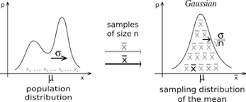
The sample average of independent and identically distributed random variables drawn from an unknown distribution with mean $\mu$ and variance $\sigma$ is approximately normal distributed when $n$ gets larger. That is, by the law of large numbers, the sample mean converges in probability and almost surely to the expected value $\mu$ as $n \to \infty$.

Formally, let ${X_1,X_2,…X_n}$ be random samples of size $n$. Then, the sample average is defined as

$$S_n = \frac{X_1 + X_2 + … + X_n}{n}$$ with mean $\mu$ and variance $\sigma^2$

Then,
$$\sqrt{n}(S_n-\mu) \sim \mathcal{N}(0,\sigma^2)$$

The normalized random mean variable will be

$$Z_n = \frac{S_n-\mu}{\frac{\sigma}{\sqrt{n}}} \sim \mathcal{N}(0,1)$$

The below part will be implementation of CLT in R.

set.seed(1004)
x1 <- runif(10000, min=0,max=1000) #Generating random variables drawn from unifrom distribution with (0,1000)

hist(x1) #Histogram

sampled.5 <- rep(0, length(x1))

for(i in 1:length(x1)){
  sampled.5[i] <- mean(sample(x1, 5, replace=TRUE)) #sample average with size 5
}

hist(sampled.5)

1 2	plot(density(sampled.5)) #density plot of sample average variables

sampled.30 <- rep(0, length(x1))
sampled.1000 <- rep(0,length(x1))
sampled.10000 <- rep(0,length(x1))

for(i in 1:length(x1)){
  sampled.30[i] <- mean(sample(x1, 30, replace=TRUE)) #sample average of size 30
  sampled.1000[i] <- mean(sample(x1, 1000, replace=TRUE)) #sample average of size 1000
  sampled.10000[i] <- mean(sample(x1,10000,replace=TRUE)) #sample average of size 10000
}

$$\sqrt{n}(S_n-\mu) \sim \mathcal{N}(0,\sigma^2)$$

The following code is the above formula.

1
2
3

sqrt(length(sampled.30))*(mean(sampled.30)-mean(x1))

## [1] -39.36105

1
2
3

sqrt(length(sampled.1000))*(mean(sampled.1000)-mean(x1))

## [1] 0.1330039

1
2
3

sqrt(length(sampled.10000))*(mean(sampled.10000)-mean(x1))

## [1] 0.003917203

It shows the $\sqrt{n}(S_n-\mu)$ tends to go to zero as the size of the sample increases, which means that the expected value of the sample average variables gets closer to the expected value of the random variables when $n$ gets larger.

Let’s see other example for random sample average drawn from Binomial distribution.

Suppose we have 10000 random Binomial variables with $p = 0.5$.

#Binomial
n <- 10000
p <- 1/2
B <- rbinom(n,1,p)

The mean of Binomial distribution is $p$, that is $E(X) = p$.
The variance of Binomial distribution is $p(1-p)$, that is $Var(X) = p(1-p)$

1
2
3

p

## [1] 0.5

1
2
3

p*(1-p)

## [1] 0.25

1
2
3

mean(B)

## [1] 0.4991

1
2
3

var(B)

## [1] 0.2500242

#creating random sample average from Binomial random variables
bin.sampled.30 <- rep(0, length(B))
bin.sampled.1000 <- rep(0,length(B))
bin.sampled.10000 <- rep(0,length(B))

for(i in 1:length(x1)){
  bin.sampled.30[i] <- mean(sample(B, 30, replace=TRUE))
  bin.sampled.1000[i] <- mean(sample(B, 1000, replace=TRUE))
  bin.sampled.10000[i] <- mean(sample(B,10000,replace=TRUE))
}

1	plot(density(bin.sampled.30))

1	plot(density(bin.sampled.1000))

1	plot(density(bin.sampled.10000))

1
2
3

sqrt(length(bin.sampled.30))*(mean(bin.sampled.30)-mean(B))

## [1] 0.009333333

1
2
3

sqrt(length(bin.sampled.1000))*(mean(bin.sampled.1000)-mean(B))

## [1] 0.01169

1
2
3

sqrt(length(bin.sampled.10000))*(mean(bin.sampled.10000)-mean(B))

## [1] -0.000371

These results shows that no matter what the distribution of the population is, the sample average drawn from the distribution will be approximately normal distribution as $n$ gets large with mean $\mu$.

Reference:
Central Limit Theorem
Central Limit Theorem (wiki)

CLT

$\large{Definition}$:

Categories

Tag Cloud

Recent

Archives

Tags

Your browser is out-of-date!