This post will discuss Central Limit Theorem.
Central Limit Theorem is one of the most important topic in statistics, especially in probability theory.

$\large{Definition}$:

The sample average of independent and identically distributed random variables drawn from an unknown distribution with mean $\mu$ and variance $\sigma$ is approximately normal distributed when $n$ gets larger. That is, by the law of large numbers, the sample mean converges in probability and almost surely to the expected value $\mu$ as $n \to \infty$.

Formally, let ${X_1,X_2,…X_n}$ be random samples of size $n$. Then, the sample average is defined as

$$S_n = \frac{X_1 + X_2 + … + X_n}{n}$$ with mean $\mu$ and variance $\sigma^2$

Then,
$$\sqrt{n}(S_n-\mu) \sim \mathcal{N}(0,\sigma^2)$$

The normalized random mean variable will be

$$Z_n = \frac{S_n-\mu}{\frac{\sigma}{\sqrt{n}}} \sim \mathcal{N}(0,1)$$

The below part will be implementation of CLT in R.

1
2
3
4

set.seed(1004)
x1 <- runif(10000, min=0,max=1000) #Generating random variables drawn from unifrom distribution with (0,1000)

hist(x1) #Histogram

1
2
3
4
5
6
7

sampled.5 <- rep(0, length(x1))

for(i in 1:length(x1)){
  sampled.5[i] <- mean(sample(x1, 5, replace=TRUE)) #sample average with size 5
}

hist(sampled.5)

1
2

plot(density(sampled.5)) #density plot of sample average variables

1
2
3
4
5
6
7
8
9

sampled.30 <- rep(0, length(x1))
sampled.1000 <- rep(0,length(x1))
sampled.10000 <- rep(0,length(x1))

for(i in 1:length(x1)){
  sampled.30[i] <- mean(sample(x1, 30, replace=TRUE)) #sample average of size 30
  sampled.1000[i] <- mean(sample(x1, 1000, replace=TRUE)) #sample average of size 1000
  sampled.10000[i] <- mean(sample(x1,10000,replace=TRUE)) #sample average of size 10000
}

$$\sqrt{n}(S_n-\mu) \sim \mathcal{N}(0,\sigma^2)$$

The following code is the above formula.

1
2
3

sqrt(length(sampled.30))*(mean(sampled.30)-mean(x1))

## [1] -39.36105

1
2
3

sqrt(length(sampled.1000))*(mean(sampled.1000)-mean(x1))

## [1] 0.1330039

1
2
3

sqrt(length(sampled.10000))*(mean(sampled.10000)-mean(x1))

## [1] 0.003917203

It shows the $\sqrt{n}(S_n-\mu)$ tends to go to zero as the size of the sample increases, which means that the expected value of the sample average variables gets closer to the expected value of the random variables when $n$ gets larger.

Let’s see other example for random sample average drawn from Binomial distribution.

Suppose we have 10000 random Binomial variables with $p = 0.5$.

1
2
3
4

#Binomial
n <- 10000
p <- 1/2
B <- rbinom(n,1,p)

The mean of Binomial distribution is $p$, that is $E(X) = p$.
The variance of Binomial distribution is $p(1-p)$, that is $Var(X) = p(1-p)$

1
2
3

p

## [1] 0.5

1
2
3

p*(1-p)

## [1] 0.25

1
2
3

mean(B)

## [1] 0.4991

1
2
3

var(B)

## [1] 0.2500242

1
2
3
4
5
6
7
8
9
10

#creating random sample average from Binomial random variables
bin.sampled.30 <- rep(0, length(B))
bin.sampled.1000 <- rep(0,length(B))
bin.sampled.10000 <- rep(0,length(B))

for(i in 1:length(x1)){
  bin.sampled.30[i] <- mean(sample(B, 30, replace=TRUE))
  bin.sampled.1000[i] <- mean(sample(B, 1000, replace=TRUE))
  bin.sampled.10000[i] <- mean(sample(B,10000,replace=TRUE))
}

1

plot(density(bin.sampled.30))

1

plot(density(bin.sampled.1000))

1

plot(density(bin.sampled.10000))

1
2
3

sqrt(length(bin.sampled.30))*(mean(bin.sampled.30)-mean(B))

## [1] 0.009333333

1
2
3

sqrt(length(bin.sampled.1000))*(mean(bin.sampled.1000)-mean(B))

## [1] 0.01169

1
2
3

sqrt(length(bin.sampled.10000))*(mean(bin.sampled.10000)-mean(B))

## [1] -0.000371

These results shows that no matter what the distribution of the population is, the sample average drawn from the distribution will be approximately normal distribution as $n$ gets large with mean $\mu$.

Reference:
Central Limit Theorem
Central Limit Theorem (wiki)

September 06th, 2019

Today’s work

1. Self-study for Gaussian Process
   • Multivariate Normal Distribution
   • Cholesky Decomposition - Generating Multivariate Normal Random Number
   • Bayesian Optimization (Fully understanding this is final goal)

Since I am going to tune hyperparameter of GBM like LightGBM or Catboost for the Kaggle Competition that I am now in, I’d like to fully understand how the Bayesian Optimization. While studying these, I have been learning more detail of matrix decomposition and Gaussian Distrubiton. I’ve also been realizing that how important they are in machine learning.

2. New Posts
   • Schur Complement
   • Cholesky Decomposition

A hard one for these posts is that I wasn’t sure how deeply I should study for them. Both of Schur Complement and Cholesky Decomposition are widely and significantly used in statistics.

2019년 9월 6일

오늘 할 일

1. Gaussian Process 셀프 스터디
   • Multivariate Normal Distribution
   • Cholesky Decomposition - Generating Multivariate Normal Random Number
   • Bayesian Optimization (Fully understanding this is final goal)

Gaussian Process 를 공부하게 된 계기는 현재 참여하고 있는 Kaggle 대회에서 LightGBM 이나 Catboost 알고리즘을 사용하려 하는데, 여기서 Hyperparameter tuning을 Random Search 나 Grid Search 가 아닌 Bayesian Optimization을 사용하기에 공부하기 시작했다.
공부하다보니 가장 기본이 되는 Matrix Decomposition, Gaussian Distribution등에 대해 더 자세히 배우고 있으며, 이들이 머신러닝에서 얼마나 많이 사용되며 중요한지 배우게 되었다.

2. 새로운 포스팅
   • Schur Complement
   • Cholesky Decomposition

이번 포스팅중 어려웠던 점은 Schur Complement과 Cholesky Decomposition은 Matrix 를 다루는 분석 혹 연구에서 매우 중요하게, 그리고 많이 쓰이기에 그 개념들을 얼마나 깊게 공부해야 하는지였다. 결국 다른 공부를 할때에도 그 개념들은 이어질테니 그때 다시 더 깊게 공부해보고 싶다.

Introduction to the Cholesky Decomposition.

Cholesky Decomposition is used for its superior efficiency in linear calculation, such as affine function, $Ax = b$. Among many applications of Cholesky Decomposition, I will discuss about how the multivariate normal random numbers are generated with Cholesky Decomposition.

$\large{Definition}$:

Every positive definite matrix $A \in \mathcal{R}^{n \times n}$,

The Cholesky Decomposition is a form of

$$A = LL^{T}$$

where $L$ is the lower triangular matrix with real and positive diagonal elements. $L$ is called Cholesky factor of $A$ and it can be interpreted as the square root of a positive definite matrix.

$\large{Algorithm}$:

This algorithm is used in this link, and there are many apporaches to decompose a matrix with Cholesky Decomposition.

1. Compute $L_{1} = \sqrt{a_{11}}$
2. For $k = 2, … ,n$, find $L_{k-1}l_{k} = a_{k} for l_{k}$
3. $l_{kk} = \sqrt{a_{kk}-l_{k}^{T}l_{k}}$
4. $L_{k} = \begin{bmatrix} L_{k-1} & 0 \\ l_{k}^{T} & l_{kk} \end{bmatrix}$

then $L_{k}$ is the lower triangular matrix of Cholesky Decomposition.

Other approaches;

• Cholesky Decomposition
• link

$\large{Generating}$ $\large{Multivariate}$ $\large{Normal}$ $\large{Random}$ $\large{Number}$ $\large{with}$ $\large{Cholesky}$ $\large{Decomposition}$

If we have $X$ that follows Normal Distribution,

then

$$X \sim \mathcal{N}(\mu, \Sigma)$$

Let $Z$ follows standard normal distribution with mean 0 and variance 1.

Then,

$$Z \sim \mathcal{N}(0,I)$$

Then, we can express the $X$ with $Z$ as the following;

$$X = A+BZ$$

then $X$ will follow normal distribution as the following;

$$X \sim \mathcal{N}(A,BB’)$$

Here, $\mu$ is the $A$, and $\Sigma$ is the $BB’$. The $B$ is the lower triangular matrix of the decomposed $X$, which is the Cholesky factor.

Therefore, If we have a Cholesky factor, $B$, of covariance matrix of $X$, then the product of $B$ and standard normal random number matrix will generate the multivariate normal random number associated with the mean $\mu$ and covariance $\Sigma$ of $X$.

Reference:

Cholesky Decomposition
Cholesky Factorization
Cholesky Decomposition with R example
link
Bivariate Normal Distribution

Brief introduction to Schur Complement.

This is just a brief introduction of the properties of Schur Complement. Schur Complement has many applications in numerical analysis, such as optimization, machine learning algorithms, or probability and matrix theories.

Let’s begin with the definition of the Schur Complement.

$\large{Definition}$:

The Schur Complement of a black matrix is defined as;

Let $M$ be $n \times n$ matrix

$$M = \begin{bmatrix} A & B \\ C & D \end{bmatrix}$$

Then, the Schur Complement of the block $D$ of the matrix $M$ is

$$M/D := A - BD^{-1}C$$

if $D$ is invertible.

The Schur Complement of the block $A$ of the matrix $M$ is then,

$$M/A := D - CA^{-1}B$$

if $A$ is invertible.

$$\large{Properties}$$

• Linear system

Let
$A$ is a $p \times p$ matrix,
$D$ is a $q \times q$ matrix, with $n = p + q$
So, $B$ is a $p \times q$ matrix.

Let $M$ be defined as,

$$M = \begin{bmatrix} A & B \\ B^{T} & D \end{bmatrix}$$

Suppose we have a linear system as,

$$Ax + By = c \\ B^{T}x + Dy = d$$

Then,

$$\begin{bmatrix} A & B \\ B^{T} & D \end{bmatrix} \begin{bmatrix} x \\ y \end{bmatrix} = \begin{bmatrix} c \\ d \end{bmatrix}$$

Assuming $D$ is invertible,

then we have $y$ as

$$y = D^{-1}(d - B^{T}x)$$

Then, from the equation,

$$Ax + By = c \\ Ax + B(D^{-1}(d - B^{T}x)) = c$$

Then, we see that is,

$$(A - BD^{-1}B^{T})x = c - BD^{-1}d$$

Here, the $A - BD^{-1}B^{T}$ is the Schur Complement of a block $D$ of matrix $M$.

It follows,

$$x = (A-BD^{-1}B^{T})^{-1}(c-BD^{-1}d) \\ y = D^{-1}(d-B^{T}(A-BD^{-1}B^{T})^{-1}(c-BD^{-1}d))$$

And,

$$x = (A-BD^{-1}B^{T})^{-1}c - (A-BD^{-1}B^{T})^{-1}BD^{-1}d \\ y = -D^{-1}B^{T}(A-BD^{-1}B^{T})^{-1}c + (D^{-1}+D^{-1}B^{T}(A-BD^{-1}B^{T})^{-1}BD^{-1})d$$

The $x$ and $y$ are formed as linear functions associated with $c$ and $d$,

and it can be a formula for an inverse of $M$ in terms of the Schur Complement of $D$ in $M$.

$$\begin{bmatrix} A & B \\ B^{T} & D \end{bmatrix} ^{-1} = \begin{bmatrix} (A-BD^{-1}B^{T})^{-1} & -(A-BD^{-1}B^{T})^{-1}BD^{-1} \\ -D^{-1}B^{T}(A-BD^{-1}B^{T})^{-1} & D^{-1}+D^{-1}B^{T}(A-BD^{-1}B^{T})^{-1}BD^{-1} \end{bmatrix}$$

This can be written as,

$$\begin{bmatrix} A & B \\ B^{T} & D \end{bmatrix} ^{-1} = \begin{bmatrix} (A-BD^{-1}B^{T})^{-1} & 0 \\ -D^{-1}B^{T}(A-BD^{-1}B^{T})^{-1} & D^{-1} \end{bmatrix} \begin{bmatrix} I & -BD^{-1} \\ 0 & I \end{bmatrix}$$

Eventually,

$$\begin{bmatrix} A & B \\ B^{T} & D \end{bmatrix} ^{-1} = \begin{bmatrix} I & 0 \\ -D^{-1}B^{T} & I \end{bmatrix} \begin{bmatrix} (A-BD^{-1}B^{T})^{-1} & 0 \\ 0 & D^{-1} \end{bmatrix} \begin{bmatrix} I & -BD^{-1} \\ 0 & I \end{bmatrix}$$

If we take inverse on both sides,

$$\begin{bmatrix} A & B \\ B^{T} & D \end{bmatrix} = \begin{bmatrix} I & BD^{-1} \\ 0 & I \end{bmatrix} \begin{bmatrix} A-BD^{-1}B^{T} & 0 \\ 0 & D \end{bmatrix} \begin{bmatrix} I & 0 \\ D^{-1}B^{T} & I \end{bmatrix}$$

$$= \begin{bmatrix} I & BD^{-1} \\ 0 & I \end{bmatrix} \begin{bmatrix} A-BD^{-1}B^{T} & 0 \\ 0 & D \end{bmatrix} \begin{bmatrix} I & BD^{-1} \\ 0 & I \end{bmatrix} ^{T}$$

This is done by an assumption with $D$ is invertible, and this decomposition is called Block LDU Decomposition.

Then, we can get another factorization of $M$ if A is invertible.

• Positive Semi-definite

For any symmetric matrix, $M$,

if D is invertible, then

1) $M \succ 0$ $iff$ $D \succ 0$ and $A-BC^{-1}B^{T} \succ 0$

2) If $C \succ 0$, then $M \succeq 0$ $iff$ $A-BC^{-1}B^{T} \succeq 0$

We can easily get the matrix $M$ in the linear combination and the inverse of the $M$ with Schur Complement.
We also can check if the $M$ is positive semi-definite.

Reference:

Schur Complement
The Schur Complement and Symmetric Positive Semidefinite (and Definite) Matrices

Logistic Regression from Logit

1. What is Logit?

To discuss logit, we need to know what the odds is.

Simply say, Odds is $\frac{p}{1-p}$, where $p$ is the probability of a binary outcome.

Since the odds has different properties than probability, it allows us to make new functions or new graphs.

With the properties of odds, logarithm of odds is popularly used in machine learning industry, which is called logit.

Logit (also log odds) = $log(\frac{p}{1-p})$.

Let logit be defined as $\theta$, then

$$\theta = log(\frac{p}{1-p})$$

We can express this in terms of $p$ as the following,

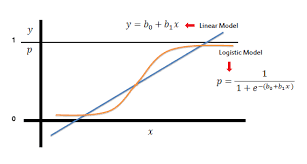
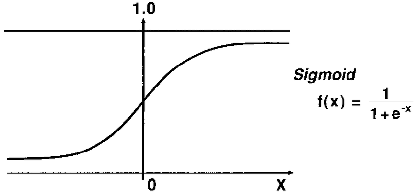
$$e^{\theta} = \frac{p}{1-p} \\ (1-p)e^{\theta} = p \\ e^{\theta} = p + p e^{\theta} \\ e^{\theta} = p(1+e^{\theta}) \\ \therefore p = \frac{e^{\theta}}{(1+e^{\theta})} = \frac{1}{1+e^{-\theta}}$$

This is the logistic function, which is the special case of sigmoid function that is widely used for classification, such as logistic regression, tree-based algorithm for classification, or deep learning.
The logistic function is the CDF of the logistic distribution.

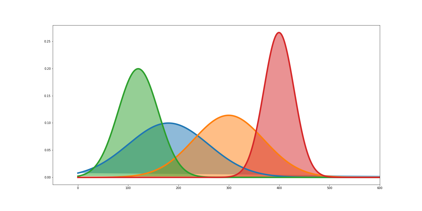
2. Logistic Distribution

A property of the logistic distribution is that the logistic distribution is very similar with the normal distribution except for the kurtosis.

The PDF of the logistic distribution is defined as,

$$f(x; \mu, s) = \frac{e^{-\frac{(x-\mu)}{s}}}{s(1+e^{-\frac{x-\mu}{s}})^2}$$

The CDF of the logistic distribution is defined as,

$$F(x; \mu, s) = \frac{1}{1+e^{-\frac{x-\mu}{s}}}$$

Some simulations are performed in this paper, and the simulation was to measure the absolute deviation between the cumulative standard normal distribution and the cumulative logistic distribution with mean zero and variance one.

By the paper, “the cumulative logistic distribution with mean zero and variance one is known as $(1+e^{-\nu x})^{-1}$ “
And, the paper also states that the kurtosis of the logistic distribution is effected by the parameter coefficient, $\nu$.
With the $\nu = 1.702$, the deviation is 0.0095.

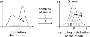
As a summary, the logistic distribution approximately follows the normal distribution with the variance $\sigma^2$, and we could use the property of the normal distribution as the following;

By wikipedia,

“If a data distribution is approximately normal, then about 68 percent of the data values are within one standard deviation of the mean (mathematically, $\mu \pm \sigma$, where $\mu$ is the arithmetic mean), about 95 percent are within two standard deviations ($\mu \pm 2\sigma$), and about 99.7 percent lie within three standard deviations ($\mu \pm 3\sigma$).”

3. Logistic Regression

In a binary logistic regression, the outcome is binary, which can be said that it follows binomial distribution.

Let $y_i$ = number of successes in $m_i$ trials of a binomial process where $i = 1,…,n$, and we have a single predictor, $x_i$.

Then,

$$y_i | x_i \sim Bin(m_i, \theta(x_i))$$

By the definition of binomial distribution,

$$P(Y_i = y_i | x_i) = \binom{m_i}{y_i}\theta(x_i)^{y_i}(1-\theta(x_i))^{m_i-y_i}$$

As I discussed in this post, Likelihood, we can find the optimal distribution for the given data.

$$\mathcal{L}(\theta | x) = \mathcal{L}(distribution | data)$$

And with the optimal distribution given by the maximum likelihood, we can predict the probability.

$$P(data | distribution)$$

Then, the likelihood function for Logistic Regression will be

$$\mathcal{L} = \prod_{i=1}^{n} P(Y_i = y_i | x_i) \\ = \prod_{i=1}^{n}\binom{m_i}{y_i}\theta(x_i)^{y_i}(1-\theta(x_i))^{m_i-y_i}$$

We take log for the likelihood function to differentiate easier because maximizing likelihood is the same with maximizing log-likelihood.

The log-likelihood function will be

$$log(\mathcal{L}) = \prod_{i=1}^{n}[log(\binom{m_i}{y_i}) + log(\theta(x_i)^{y_i}) + log((1-\theta(x_i))^{m_i - y_i})] \\ = \prod_{i=1}^{n}[y_{i} log(\theta(x_i)) + (m_i - y_i)log(1-\theta(x_i)) + log(\binom{m_i}{y_i})] \\ = \prod_{i=1}^{n}[y_{i} log(\frac{\theta(x_i)}{1-\theta(x_i)}) + m_{i} log(1-\theta(x_i)) + log(\binom{m_i}{y_i})] \\ = \prod_{i=1}{n}[y_{i}(\beta_{0} + \beta_{1}x_{i}) - m_{i}log(1+exp(\beta_{0}+\beta_{1}x_{i})) + log(\binom{m_i}{y_i})]$$

Here, the $\theta(x_i)$, which is the probability, is defined as

$$\theta(x_i) = \frac{1}{1+e^{-(\beta_0 + \beta_1 x_i)}}$$

And, the linear combination of $\beta$ and $x$ will be the log odds as the following,

$$log(\frac{\theta(x_i)}{1-\theta(x_i)}) = \beta_0 + \beta_1 x_i$$

Just taking the derivative on the log-likelihood function and setting this as zero is hard to solve the problem, so the parameter $\beta_0$ and $\beta_1$ can be estimated by some other optimization method, such as Newton’s method.

4. Wald Test in Logistic Regression

Wald Test uses the property of the logistic distribution.

As mentioned above, the logistic distribution is almost approximately standard normal distribution.

Hence, the Wald test statistic is used to test

$$H_0 : \beta_1 = 0$$

in Logistic regression.

The Wald test statistic is defined as

$$Z = \frac{\hat{\beta_1} - \beta_1}{estimated \qquad se(\hat{\beta_1})}$$

In the test, $\beta_1 = 0$ as the null hypothesis, and this follows standard normal distribution.

Hence,

$$Z = \frac{\hat{\beta_1}}{\hat{se}(\hat{\beta_1})} \sim \mathcal{N}(0,1)$$

As mentioned above, the logistic distribution is approximately following the normal distribution with variance, $\sigma^2$.
Hence, dividing by the standard error for the estimated paramter gives you standard normal distribution, $\mathcal{N}(0,1)$.

We can determine the coefficient significant with the Wald Test for the Logistic Regression.

4. Interpretation for coefficients of Logistic Regression.

Unlike Linear Regression, the linear combination of coefficients of Logistic regression is logit.

Hence, we can interpret the coefficient in different way.

For example, with the single predictor as used above, the logit is

$$log(\frac{p}{1-p}) = \beta_0 + \beta_1 x_i$$

If we take exponential both sides,

$$\frac{p}{1-p} = e^{(\beta_0 + \beta_1 x_i)}$$

Then, we can say as following,

“For one-unit in $x_i$ increase, it is expected to see ..% increase in odds of success, $p$”.

Reference:
A Modern Approach to Regression With R by Simon J. Sheater, Springer
A logistic approximation to the cumulative normal distribution
Standard Deviation
Logistic Distribution

Likelihood vs Probability

Likelihood Definition (Wikipedia) : In statistics, the likelihood function expresses how probable a given set of observations is for different values of statistical parameters. It is equal to the joint probability distribution of the random sample evaluated at the given observations, and it is, thus, solely a functoin of paramters that index the family of those probability distributions.

1. What is Likelihood?

Likelihoods are the y-axis values for fixed data points with distribution that can be moved, as the following;

$$\mathcal{L}(\theta | x) = \mathcal{L}(distribution | data)$$

Whereas, Probabilities are the areas under a fixed distribution.

$$P(data | distribution)$$

If we find the maximum y-axis value for fixed data points by moving the distribution, we find the optimal distribution for the fixed data.
Therefore, we can use the likelihood function to fit a optimal distribution on the fixed data by finding maximum likelihood estimator.

2. Maximum Likelihood?

To find the maximum likelihood estimator, we might find a function for likelihoods given fixed data points, and take a derivative for the function, and set the derivatives as 0.

Example 1: Exponential distribution

The Probability Density Function of Exponential Distribution is defined as the following;

$$f(x; \lambda) = \lambda e ^ {- \lambda x} \qquad if \qquad x \geq 0$$

Otherwise,

$$f(x; \lambda) = 0$$

for $\lambda >0$, which is rate parameter of the distribution.

Hence, the exponential distribution will be shaped by the $\lambda$.

Therefore, we want to find the maximum likelihood of $\lambda$ for given data.

$$\mathcal{L}(\lambda | x_1, x_2, … , x_n) = \mathcal{L}(\lambda | x_1)\mathcal{L}(\lambda | x_2)…\mathcal{L}(\lambda | x_n) $$

$$= \lambda e ^ {- \lambda x_1}\lambda e ^ {- \lambda x_2}…\lambda e ^ {- \lambda x_n} \\ = \lambda^{n}(e ^ {-\lambda (x_1 + x_2 + … + x_n)})$$

Now, take a derivative for the likelihood function to find maximum likelihood estimator of $\lambda$.

$$ \frac{d}{d\lambda} \mathcal{L}(\lambda | x_1, x_2, … , x_n) = \frac{d}{d\lambda} \lambda^{n} (e ^ {-\lambda * (x_1 + x_2 + … + x_n)})$$

Before derivitaves, there is more easier way to differentiate this function, which is to take a lograithm on the function.
Take a logarithm on the likelihood function, then this becomes the log likelihood function.

$$log (\mathcal{L}(\lambda | x_1, x_2, … , x_n)) = log(\mathcal{L}(\lambda | x_1)\mathcal{L}(\lambda | x_2)…\mathcal{L}(\lambda | x_n))
$$

Which makes easier differentiate the function.

$$ \frac{d}{d\lambda} log(\mathcal{L}(\lambda | x_1, x_2, … , x_n)) = \frac{d}{d\lambda} log(\lambda^{n}(e ^ {-\lambda * (x_1 + x_2 + … + x_n)}))$$

$$= \frac{d}{d\lambda} (log(\lambda ^ {n}) + log(\lambda^{n}(e ^ {-\lambda * (x_1 + x_2 + … + x_n)}))) \\ = \frac{d}{d\lambda} (n log(\lambda) - \lambda (x_1 + x_2 + … + x_n)) \\ = n \frac{1}{\lambda} - (x_1 + x_2 + … + x_n)$$

Set this as zero,

$$n \frac{1}{\lambda} - (x_1 + x_2 + … + x_n) = 0$$

Which gives you,

$$ \frac{(x_1 + x_2 + … + x_n)}{n} = \mu = \frac{1}{\lambda}$$

Therefore, the maximum likelihood estimator of $\lambda$ is

$$\lambda = \frac{1}{\mu}$$.

And, this connects to the concept of the maximum entropy probability distribution.

“The exponential distribution is the maximum entropy distribution among all continuous distribution supported in $[0, \infty]$ that have a specified mean of $\frac{1}{\lambda}$”

Example 2: Normal Distribution

In normal distribution (often called Gaussian distribution), the mean $\mu$ and the variance $\sigma^2$ will be the parameter that the determines how the normal distribution looks like. With $\mu$ and $\sigma^2$, we will find the maximum likelihood estimator for the normal distribution given fixed data.

The PDF of normal distribution is defined as,

$$f(x|\mu, \sigma^2) = \frac{1}{\sqrt{2\pi\sigma^2}} e^{-\frac{(x-\mu)^2}{2\sigma^2}}$$

The Likelihood of $\mu$ and $\sigma$ for normal distribution will be,

$$\mathcal{L}(\mu, \sigma|x_1, x_2, … , x_n) = \mathcal{L}(\mu, \sigma^2|x_1)\mathcal{L}(\mu, \sigma^2|x_2)…\mathcal{L}(\mu, \sigma^2|x_n)$$

$$= \frac{1}{\sqrt{2\pi\sigma^2}} e^{-\frac{(x_1-\mu)^2}{2\sigma^2}}\frac{1}{\sqrt{2\pi\sigma^2}} e^{-\frac{(x_2-\mu)^2}{2\sigma^2}}…\frac{1}{\sqrt{2\pi\sigma^2}} e^{-\frac{(x_n-\mu)^2}{2\sigma^2}}$$

Before take a derivatives, we take a log on the function as done in exponential.

$$log(\mathcal{L}(\mu, \sigma|x_1, x_2, … , x_n))= log(\frac{1}{\sqrt{2\pi\sigma^2}} e^{-\frac{(x_1-\mu)^2}{2\sigma^2}}\frac{1}{\sqrt{2\pi\sigma^2}} e^{-\frac{(x_2-\mu)^2}{2\sigma^2}}…\frac{1}{\sqrt{2\pi\sigma^2}} e^{-\frac{(x_n-\mu)^2}{2\sigma^2}})$$

By simplifying the log likelihood function with the properties of logarithm,

$$= \sum_{i=1}^{n}(log(\frac{1}{\sqrt{2\pi\sigma^2}}) -\frac{(x_i-\mu)^2}{2\sigma^2}) \\ = -\frac{n}{2}log(2\pi) - nlog(\sigma) - \sum_{i=1}^{n}\frac{(x_i-\mu)^2}{2\sigma^2}$$

Now, take the derivative with respect to the $\mu$,

$$\frac{\partial}{\partial \mu} log(\mathcal{L}(\mu, \sigma|x_1, x_2, … , x_n)) \\ = 0 - 0 + \sum_{i=1}^{n} \frac{(x_i-\mu)}{\sigma^2} \\ = \sum_{i=1}^{n} \frac{x_i}{\sigma^2} - n\mu$$

Set this as 0,

$$\sum_{i=1}^{n} \frac{x_i}{\sigma^2} - n\mu = 0$$

Since $\sigma^2$ is constant here,

$$ \sum_{i=1}^{n} x_i = n\mu$$

Hence,

$$\mu = \sum_{i=1}^{n} x_i / n$$
which is the mean of the measurements.

Taking derivative with respect to the $\sigma$,

$$\frac{\partial}{\partial \sigma} log(\mathcal{L}(\mu, \sigma|x_1, x_2, … , x_n)) = \frac{\partial}{\partial \sigma} (-\frac{n}{2}log(2\pi) - nlog(\sigma) - \sum_{i=1}^{n}\frac{(x_i-\mu)^2}{2\sigma^2}) \\ = 0 - \frac{n}{\sigma} + \sum_{i=1}^{n} \frac{(x_i - \mu)^2}{\sigma^3}$$

Set this as 0,

$$0 - \frac{n}{\sigma} + \sum_{i=1}^{n} \frac{(x_i - \mu)^2}{\sigma^3} = 0 \\ n = \sum_{i=1}^{n} \frac{(x_i - \mu)^2}{\sigma^2} \\ \sigma^2 = \sum_{i=1}^{n} \frac{(x_i - \mu)^2}{n} \\ \sigma = \sum_{i=1}^{n} \sqrt{\frac{(x_i - \mu)^2}{n}}$$
which is the standard deviation of the measurements.

In conclusion,

the mean of the data is the maximum likelihood estimate for where the center of the distribution should be,

the standard deviation of the data is the maximum likelihood estimate for how wide the curve of the distribution should be.

This also connects to the maximum entropy probability distribution as the following;

The normal distribution has maximum entropy among all real-valued distribution supported on $(-\infty, \infty)$ with a specified variance $\sigma^2$.

Reference:
Likelihood(wiki)
Maximum Entropy Probability Distribution(wiki)
Related to Likelihood for distributions (StatQuest with Josh Starmer)

August 28th, 2019

Today’s work

1. Convex Optimization Course - Duality;
   weak and strong duality
2. IEEE Kaggle - Data Organization;
   convert data by Data Description - link
3. Study LightGBM with the video presented by Mateusz Susik from McKinsey - link

XGBoost by Tianqi Chen- link

오늘 할 일

1. Convex Optimization 수업 - Duality; weak and strong duality
2. IEEE 카글 대회 - 데이터 정리; 데이터 Description에 따라 변수들 변환 - link
3. LightGBM 원리 공부 - 프레젠테이션 Mateusz Susik from McKinsey - link

XGBoost -> LightGBM

Update:

Duality -

1. Form Lagrange

   $\mathcal{L}(x,\lambda,\nu)$ = $f_0 (x) + \sum_{i=1}^{m} \lambda_i f_i(x) + \sum_{i=1}^{p} \nu_i h_i (x)$

2. Set gradient for $x$ equal to zero to minimize $\mathcal{L}$

   $\nabla_x \mathcal{L}$ = 0

3. Plug it in $\mathcal{L}$ to get the Lagrangian dual function;

   $g(\lambda, \nu)$ = $\inf_{x\in D} \mathcal{L}(x, \lambda, \nu)$

   which is a concave function, can be $-\infty$ for some $\lambda, \nu$

   Lagrangian dual function is a concave function, since the Lagrangian form is affine function, and infimum of any family of affine is concave.

   We want to maximize lower bound (concave) to get the best optimal points, and maximizing lower bound is convex optimization problem.

LightGBM - XGBoost (either histogram implementation available)

One of the method used in LightGBM is ‘Graident-based one-side sampling’ that is the biggest benefit of LightGBM. This method is to concentrate on data points with large gradients and ignore data points with small graidents (close to local minima).

LightGBM - XGBoost(둘 다 histogram implementation 가능)

가장 큰 장점은 Gradient-based one-side sampling 이라는 방법으로, gradient가 큰 데이터 포인트들을 집중하며, small gradients (Gradients가 작다는 것은 local minima에 가깝다는것이고, 그 말은 즉 Residual 혹은 loss 가 적다는것) 들은 무시하기에 training 속도가 굉장히 빠르다는 것.

Welcome to David’s blog!
I am excited to start my first blog.

This is Yongbock (David) Kwon who likes studying statistics, especially machine learning.

I love to listen to musics!

I started this blog to record what I study, what I listen to, and what I think in my daily life, because I have a bad memory.

And, the record is the one that is able to get over against the river of time as a human.

Hence, this blog will be my study notes, my diary, and the representation of myself.

Let’s begin!

제 블로그에 오신걸 환영합니다!
첫 블로그인지라 많이 긴장되네요!

현재 머신러닝을 공부중에 있으며, 음악듣는걸 좋아합니다.

기억력이 좋지 않은 편이라, 무엇을 공부했고, 무슨 음악을 들으며, 일상중에 무슨 생각을 하는지에 대해 기록해보고자 블로그를 만들었습니다.

즉, 제 공부 노트이자, 일기장이자, 권용복이 누구인지 보여주는 블로그입니다!