Creating Histogram function using Min-max transformation.

The histogram plot of a vector or a data feature is to create bins, which is to create a series of interval, for the range of data values, and to count how many data values fall into each bins.

I create bins as the following;

Suppose we have $M$ bins, then

$$B_1 = [0,\frac{1}{M}), B_2 = [\frac{1}{M}, \frac{2}{M}), …, B_{M-1} = [\frac{M-2}{M}, \frac{M-1}{M}), B_{M} = [\frac{M-1}{M}, 1)$$

To create histogram function with the bins, I wanted to transform the data elements in interval $(0,1)$, so I can put them into each bins.

That’s why I used Min-max transformation, which makes the data reducing to a scale between 0 and 1.

Min-max transformation is the following formula;

$$z = \frac{x-min(x)}{max(x)-min(x)}$$

The below codes are the implementation of creating histogram plot in R. I used the values from CLT posts.

CLT link

1
2
3
4
5
6
7
8
9
10
11
12
13
14
15
16
17
18
19
20
21

Hist <- function(vec,bin){
  vec.minmax <- (vec - min(vec))/(max(vec)-min(vec)) #min-max transformation of the vector or the values
  
  vec.bins <- rep(0,bin)
  for(i in 1:bin){
  	#find the values that is the closest to the value of each boundary of the bins
    vec.bins[i] <- vec[which(abs(vec.minmax - i/bin) == min(abs(vec.minmax - i/bin)))]
  }
  
  dat <- data.frame(x=vec.bins, freq=0)
  for(i in 1:bin){
  	#put the values into each bins associateed
    dat[i,2] <- length(which(vec.minmax > (i-1)/bin & vec.minmax <= i/bin))
  }
  
  #plotting
  p <- dat %>% ggplot(aes(x=x, y=freq)) + geom_bar(stat="identity", position=position_dodge(width=0.5)) + theme_bw()

  return(p)
}

1

Hist(sampled.1000,15)

1

Hist(sampled.10000,15)

1

Hist(bin.sampled.10000,15)

Reference:
Histogram and Kernel Density EStimation
Histogram from Scratch

This post will discuss Central Limit Theorem.
Central Limit Theorem is one of the most important topic in statistics, especially in probability theory.

$\large{Definition}$:

The sample average of independent and identically distributed random variables drawn from an unknown distribution with mean $\mu$ and variance $\sigma$ is approximately normal distributed when $n$ gets larger. That is, by the law of large numbers, the sample mean converges in probability and almost surely to the expected value $\mu$ as $n \to \infty$.

Formally, let ${X_1,X_2,…X_n}$ be random samples of size $n$. Then, the sample average is defined as

$$S_n = \frac{X_1 + X_2 + … + X_n}{n}$$ with mean $\mu$ and variance $\sigma^2$

Then,
$$\sqrt{n}(S_n-\mu) \sim \mathcal{N}(0,\sigma^2)$$

The normalized random mean variable will be

$$Z_n = \frac{S_n-\mu}{\frac{\sigma}{\sqrt{n}}} \sim \mathcal{N}(0,1)$$

The below part will be implementation of CLT in R.

1
2
3
4

set.seed(1004)
x1 <- runif(10000, min=0,max=1000) #Generating random variables drawn from unifrom distribution with (0,1000)

hist(x1) #Histogram

1
2
3
4
5
6
7

sampled.5 <- rep(0, length(x1))

for(i in 1:length(x1)){
  sampled.5[i] <- mean(sample(x1, 5, replace=TRUE)) #sample average with size 5
}

hist(sampled.5)

1
2

plot(density(sampled.5)) #density plot of sample average variables

1
2
3
4
5
6
7
8
9

sampled.30 <- rep(0, length(x1))
sampled.1000 <- rep(0,length(x1))
sampled.10000 <- rep(0,length(x1))

for(i in 1:length(x1)){
  sampled.30[i] <- mean(sample(x1, 30, replace=TRUE)) #sample average of size 30
  sampled.1000[i] <- mean(sample(x1, 1000, replace=TRUE)) #sample average of size 1000
  sampled.10000[i] <- mean(sample(x1,10000,replace=TRUE)) #sample average of size 10000
}

$$\sqrt{n}(S_n-\mu) \sim \mathcal{N}(0,\sigma^2)$$

The following code is the above formula.

1
2
3

sqrt(length(sampled.30))*(mean(sampled.30)-mean(x1))

## [1] -39.36105

1
2
3

sqrt(length(sampled.1000))*(mean(sampled.1000)-mean(x1))

## [1] 0.1330039

1
2
3

sqrt(length(sampled.10000))*(mean(sampled.10000)-mean(x1))

## [1] 0.003917203

It shows the $\sqrt{n}(S_n-\mu)$ tends to go to zero as the size of the sample increases, which means that the expected value of the sample average variables gets closer to the expected value of the random variables when $n$ gets larger.

Let’s see other example for random sample average drawn from Binomial distribution.

Suppose we have 10000 random Binomial variables with $p = 0.5$.

1
2
3
4

#Binomial
n <- 10000
p <- 1/2
B <- rbinom(n,1,p)

The mean of Binomial distribution is $p$, that is $E(X) = p$.
The variance of Binomial distribution is $p(1-p)$, that is $Var(X) = p(1-p)$

1
2
3

p

## [1] 0.5

1
2
3

p*(1-p)

## [1] 0.25

1
2
3

mean(B)

## [1] 0.4991

1
2
3

var(B)

## [1] 0.2500242

1
2
3
4
5
6
7
8
9
10

#creating random sample average from Binomial random variables
bin.sampled.30 <- rep(0, length(B))
bin.sampled.1000 <- rep(0,length(B))
bin.sampled.10000 <- rep(0,length(B))

for(i in 1:length(x1)){
  bin.sampled.30[i] <- mean(sample(B, 30, replace=TRUE))
  bin.sampled.1000[i] <- mean(sample(B, 1000, replace=TRUE))
  bin.sampled.10000[i] <- mean(sample(B,10000,replace=TRUE))
}

1

plot(density(bin.sampled.30))

1

plot(density(bin.sampled.1000))

1

plot(density(bin.sampled.10000))

1
2
3

sqrt(length(bin.sampled.30))*(mean(bin.sampled.30)-mean(B))

## [1] 0.009333333

1
2
3

sqrt(length(bin.sampled.1000))*(mean(bin.sampled.1000)-mean(B))

## [1] 0.01169

1
2
3

sqrt(length(bin.sampled.10000))*(mean(bin.sampled.10000)-mean(B))

## [1] -0.000371

These results shows that no matter what the distribution of the population is, the sample average drawn from the distribution will be approximately normal distribution as $n$ gets large with mean $\mu$.

Reference:
Central Limit Theorem
Central Limit Theorem (wiki)

Introduction to the Cholesky Decomposition.

Cholesky Decomposition is used for its superior efficiency in linear calculation, such as affine function, $Ax = b$. Among many applications of Cholesky Decomposition, I will discuss about how the multivariate normal random numbers are generated with Cholesky Decomposition.

$\large{Definition}$:

Every positive definite matrix $A \in \mathcal{R}^{n \times n}$,

The Cholesky Decomposition is a form of

$$A = LL^{T}$$

where $L$ is the lower triangular matrix with real and positive diagonal elements. $L$ is called Cholesky factor of $A$ and it can be interpreted as the square root of a positive definite matrix.

$\large{Algorithm}$:

This algorithm is used in this link, and there are many apporaches to decompose a matrix with Cholesky Decomposition.

1. Compute $L_{1} = \sqrt{a_{11}}$
2. For $k = 2, … ,n$, find $L_{k-1}l_{k} = a_{k} for l_{k}$
3. $l_{kk} = \sqrt{a_{kk}-l_{k}^{T}l_{k}}$
4. $L_{k} = \begin{bmatrix} L_{k-1} & 0 \\ l_{k}^{T} & l_{kk} \end{bmatrix}$

then $L_{k}$ is the lower triangular matrix of Cholesky Decomposition.

Other approaches;

• Cholesky Decomposition
• link

$\large{Generating}$ $\large{Multivariate}$ $\large{Normal}$ $\large{Random}$ $\large{Number}$ $\large{with}$ $\large{Cholesky}$ $\large{Decomposition}$

If we have $X$ that follows Normal Distribution,

then

$$X \sim \mathcal{N}(\mu, \Sigma)$$

Let $Z$ follows standard normal distribution with mean 0 and variance 1.

Then,

$$Z \sim \mathcal{N}(0,I)$$

Then, we can express the $X$ with $Z$ as the following;

$$X = A+BZ$$

then $X$ will follow normal distribution as the following;

$$X \sim \mathcal{N}(A,BB’)$$

Here, $\mu$ is the $A$, and $\Sigma$ is the $BB’$. The $B$ is the lower triangular matrix of the decomposed $X$, which is the Cholesky factor.

Therefore, If we have a Cholesky factor, $B$, of covariance matrix of $X$, then the product of $B$ and standard normal random number matrix will generate the multivariate normal random number associated with the mean $\mu$ and covariance $\Sigma$ of $X$.

Reference:

Cholesky Decomposition
Cholesky Factorization
Cholesky Decomposition with R example
link
Bivariate Normal Distribution

Brief introduction to Schur Complement.

This is just a brief introduction of the properties of Schur Complement. Schur Complement has many applications in numerical analysis, such as optimization, machine learning algorithms, or probability and matrix theories.

Let’s begin with the definition of the Schur Complement.

$\large{Definition}$:

The Schur Complement of a black matrix is defined as;

Let $M$ be $n \times n$ matrix

$$M = \begin{bmatrix} A & B \\ C & D \end{bmatrix}$$

Then, the Schur Complement of the block $D$ of the matrix $M$ is

$$M/D := A - BD^{-1}C$$

if $D$ is invertible.

The Schur Complement of the block $A$ of the matrix $M$ is then,

$$M/A := D - CA^{-1}B$$

if $A$ is invertible.

$$\large{Properties}$$

• Linear system

Let
$A$ is a $p \times p$ matrix,
$D$ is a $q \times q$ matrix, with $n = p + q$
So, $B$ is a $p \times q$ matrix.

Let $M$ be defined as,

$$M = \begin{bmatrix} A & B \\ B^{T} & D \end{bmatrix}$$

Suppose we have a linear system as,

$$Ax + By = c \\ B^{T}x + Dy = d$$

Then,

$$\begin{bmatrix} A & B \\ B^{T} & D \end{bmatrix} \begin{bmatrix} x \\ y \end{bmatrix} = \begin{bmatrix} c \\ d \end{bmatrix}$$

Assuming $D$ is invertible,

then we have $y$ as

$$y = D^{-1}(d - B^{T}x)$$

Then, from the equation,

$$Ax + By = c \\ Ax + B(D^{-1}(d - B^{T}x)) = c$$

Then, we see that is,

$$(A - BD^{-1}B^{T})x = c - BD^{-1}d$$

Here, the $A - BD^{-1}B^{T}$ is the Schur Complement of a block $D$ of matrix $M$.

It follows,

$$x = (A-BD^{-1}B^{T})^{-1}(c-BD^{-1}d) \\ y = D^{-1}(d-B^{T}(A-BD^{-1}B^{T})^{-1}(c-BD^{-1}d))$$

And,

$$x = (A-BD^{-1}B^{T})^{-1}c - (A-BD^{-1}B^{T})^{-1}BD^{-1}d \\ y = -D^{-1}B^{T}(A-BD^{-1}B^{T})^{-1}c + (D^{-1}+D^{-1}B^{T}(A-BD^{-1}B^{T})^{-1}BD^{-1})d$$

The $x$ and $y$ are formed as linear functions associated with $c$ and $d$,

and it can be a formula for an inverse of $M$ in terms of the Schur Complement of $D$ in $M$.

$$\begin{bmatrix} A & B \\ B^{T} & D \end{bmatrix} ^{-1} = \begin{bmatrix} (A-BD^{-1}B^{T})^{-1} & -(A-BD^{-1}B^{T})^{-1}BD^{-1} \\ -D^{-1}B^{T}(A-BD^{-1}B^{T})^{-1} & D^{-1}+D^{-1}B^{T}(A-BD^{-1}B^{T})^{-1}BD^{-1} \end{bmatrix}$$

This can be written as,

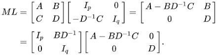
$$\begin{bmatrix} A & B \\ B^{T} & D \end{bmatrix} ^{-1} = \begin{bmatrix} (A-BD^{-1}B^{T})^{-1} & 0 \\ -D^{-1}B^{T}(A-BD^{-1}B^{T})^{-1} & D^{-1} \end{bmatrix} \begin{bmatrix} I & -BD^{-1} \\ 0 & I \end{bmatrix}$$

Eventually,

$$\begin{bmatrix} A & B \\ B^{T} & D \end{bmatrix} ^{-1} = \begin{bmatrix} I & 0 \\ -D^{-1}B^{T} & I \end{bmatrix} \begin{bmatrix} (A-BD^{-1}B^{T})^{-1} & 0 \\ 0 & D^{-1} \end{bmatrix} \begin{bmatrix} I & -BD^{-1} \\ 0 & I \end{bmatrix}$$

If we take inverse on both sides,

$$\begin{bmatrix} A & B \\ B^{T} & D \end{bmatrix} = \begin{bmatrix} I & BD^{-1} \\ 0 & I \end{bmatrix} \begin{bmatrix} A-BD^{-1}B^{T} & 0 \\ 0 & D \end{bmatrix} \begin{bmatrix} I & 0 \\ D^{-1}B^{T} & I \end{bmatrix}$$

$$= \begin{bmatrix} I & BD^{-1} \\ 0 & I \end{bmatrix} \begin{bmatrix} A-BD^{-1}B^{T} & 0 \\ 0 & D \end{bmatrix} \begin{bmatrix} I & BD^{-1} \\ 0 & I \end{bmatrix} ^{T}$$

This is done by an assumption with $D$ is invertible, and this decomposition is called Block LDU Decomposition.

Then, we can get another factorization of $M$ if A is invertible.

• Positive Semi-definite

For any symmetric matrix, $M$,

if D is invertible, then

1) $M \succ 0$ $iff$ $D \succ 0$ and $A-BC^{-1}B^{T} \succ 0$

2) If $C \succ 0$, then $M \succeq 0$ $iff$ $A-BC^{-1}B^{T} \succeq 0$

We can easily get the matrix $M$ in the linear combination and the inverse of the $M$ with Schur Complement.
We also can check if the $M$ is positive semi-definite.

Reference:

Schur Complement
The Schur Complement and Symmetric Positive Semidefinite (and Definite) Matrices