Logistic Regression - Newton's method

Logistic Regression Algorithm with Newton’s Method

This post will somehow overlap the previous post, Logistic Regression I, since I will discuss about the Logistic Regression further the post.

We start with the Binomial Distribution.

Binomial Distribution

Let $Y$ be the number of success in $m$ trials of a binomial process. Then Y is said to have a binomial distribution with paramters of $m$ and $\theta$.

$$Y \sim Bin(m, \theta)$$

The probability that $Y$ takes the integer value $j$ ($j = 0, 1, …, m$) is given by,

$$P(Y = j) = \binom{m}{j} \theta^j (1-\theta)^{m-j}$$

Then, let $y_i$ be the number of success in $m_i$ trials of a binomial process where $i = 1, …, n$.

$$(Y = y_i|X = x_i) \sim Bin(m_i, \theta(x_i))$$

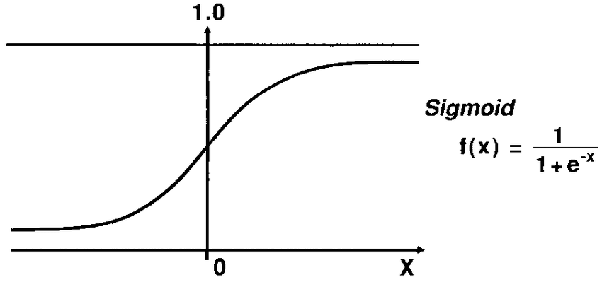
Sigmoid Function

In logistic regression for binary response variable, we use sigmoid function to figure out the optimization of loss function, or cost function, of logistic regression model because the sigmoid function can be differentiated.

Let we have one predictor variable, $x$, to predict binary outcome variable.

Then, sigmoid function is defined as below,

$$\theta(x) = \frac{e^{\beta_0 + \beta_1x}}{1 + e^{\beta_0 + \beta_1x}} = \frac{1}{1 + e^{-(\beta_0 + \beta_1x)}}$$

Here, the $\theta(x)$ is the probability of success.
Solving the equation for $\beta_0 + \beta_1x$,

$$\beta_0 + \beta_1x = log(\frac{\theta(x)}{1-\theta(x)}) $$
Here, the $\frac{\theta(x)}{1-\theta(x)}$ is known as odds, which can be described as “odds in favor of success”

The odds can be described as,

$$odds = \frac{Probability}{1-Probability}$$

As the previous posts, Logistic Regression I and Likelihood discussed, the likelihood and the probability in the dataset can be seen as,

$$\mathcal{L}(\theta | x) = \mathcal{L}(distribution | data)$$

$$P(data | distribution)$$

Then, if we find the optimal distribution given by the maximum likelihood or the minimum loss function, we can find the probability of the outcome.

Likelihood of Logistic Regression

Let $\theta(X) = \frac{1}{1+e^{-(X\beta)}}$, then the likelihood function is the function of the unkown probability of success $\theta(X)$ given by..

$$L = \prod_{i=1}^{n} P(Y_i = y_i|X = x_i) \\ = \prod_{i=1}^{n} \binom{m_i}{y_i} \theta(x_i)^{y_i} (1-\theta(x_i))^{m_i - y_i}$$

To simplify the likelihood, we take the log on the equation,

$$log(L) = \sum_{i=1}^{n}[log(\binom{m_i}{y_i}) + log(\theta(x_i)^{y_i}) + log((1-\theta(x_i))^{m_i - y_i})] \\ = \sum_{i=1}^{n}[y_ilog(\theta(x_i)) + (m_i-y_i)log(1-\theta(x_i)) + log(\binom{m_i}{y_i})] $$

Here, the all $m_i$ is equal to 1 for the binary outcome variable. Therefore,

$$log(L) = \sum_{i=1}^{n}[y_ilog(\theta(x_i)) + (1-y_i)log(1-\theta(x_i))] \tag{Eq 1}$$

The constant, $log(\binom{m_i}{y_i})$ is excluded here, since it won’t affect in optimization. The equation $(Eq 1)$ is the log likelihood function that we want to maximize. We take the minus sign for the log likelihood, which is the cost function of logistic regression.

Then, the cost function for Logistic regression is the normalization of the negative log likelihood function, which is the final cost function that we want to minimize.

$$J = -\frac{1}{n}\sum_{i=1}^{n}[y_ilog(\theta(x_i)) + (1-y_i)log(1-\theta(x_i))] \tag{Eq 2}$$

Newton-Raphson Method

This optimization method is often called as Newton’s method, and the form is given by,

$$\theta_{k+1} = \theta_k - H_k^{-1}g_k$$

where $H_k$ is the Hessian matrix, which is the second partial derivative matrix, and $g_k$, which is the first partial derivative matrix, is the gradient matrix.

It comes from the Taylor approximation of $f(\theta)$ around $\theta_k$.

$$f_{quad}(\theta) = f(\theta_k) + g_k^{T}(\theta - \theta_k) + \frac{1}{2}(\theta - \theta_k)^{T}H_k(\theta - \theta_k)$$

Setting the derivative of the function for $\theta$ equal to 0 to find the critical point.

$$\frac{\partial f_{quad}(\theta)}{\partial \theta} = 0 + g_k + H_k(\theta - \theta_k) = 0 \\ -g_k = H_k(\theta-\theta_k) \\ = H_k\theta - H_k\theta_k \\ H_k\theta = H_k\theta_k - g_k \\ \therefore \theta_{k+1} = \theta_k - H_k^{-1}g_k $$

Linear Regression with Newton-Raphson Method

In linear regression, the $\hat y$ is given by $X\theta$, and therefore, least squares, which is the cost function, is given by ..

$$f(\theta) = f(\theta; X, y) = (y-X\theta)^{T}(y-X\theta) \\ = y^Ty - y^TX\theta - \theta^TX^Ty + \theta^TX^TX\theta \\ = y^Ty - 2\theta^TX^Ty + \theta^TX^TX\theta$$

Then, the gradient is..

$$g = \partial f(\theta) = -2X^T y + 2X^T X \theta$$

The Hessian is..

$$H = \partial^2f(\theta) = 2X^TX $$

The Newton’s method for Linear Regression is..

$$\therefore \theta_{k+1} = \theta_k - H_k^{-1}g_k \\ = \theta_k - (2X^TX)^{-1}(-2X^Ty + 2X^TX\theta_k) \\ = \theta_k + (X^TX)^{-1}(X^Ty) - (X^TX)^{-1}X^TX\theta_k \\ \therefore \hat \beta= (X^TX)^{-1}X^Ty $$

Logistic Regression with Newton’s method

Recall that the cost function for logistic regression is described as $(Eq 2)$,

$$J = -\frac{1}{n}\sum_{i=1}^{n}[y_ilog(\theta(x_i)) + (1-y_i)log(1-\theta(x_i))] $$

Therefore, the gradient of the cost function is given by

$$g = X^T(\theta(X) - y)$$

the Hessian is given by

$$ X^TWX $$

Then, the $\beta$ is given by the Newton’s method

$$\theta_{k+1} = \theta_k - H_k^{-1}g_k \\ = \theta_k - (X^TWX)^{-1}(X^T(\theta_k(X) - y)) \\ \therefore \hat \beta = \theta_k - (X^TWX)^{-1}(X^T(\theta_k(X) - y))$$

Calculation of the results

The standard error for the coefficients are the square root of the diagonal elements of the Hessian matrix.

The z value is the

$$Z = \frac{\hat \beta}{estimated \qquad se(\hat \beta)}$$

and this statistic is used to test if $\beta = 0$, and it’s called a Wald test statistic.

As I dealt with the similarity of the logit with the standard normal distribution in the previous post, Logistic Regression I, we can use this statistic to test for statistical significance. The confidence interval can be calculated by

$$\hat \beta \pm z_{1-\alpha/2} \hat {se}(\hat \beta)$$

Implementation

1
2
3
4
5
6
7
8
9
10
11
12
13
14
15
16
17
18
19
20
21
22
23
24
25
26
27
28
29
30
31
32
33
34
35
36
37
38
39
40
41
42
43
44
45
46
47
48
49
50
51
52
53
54
55
56
57
58
59
60
61
62
63
64
65
66
67
68
69

#Sigmoid function - make cost function derivative
sigmoid <- function(lo){
  sig <- 1/(1+exp(-lo))
  return(sig)
}

#cost function - mean of negative log likelihood function
LL.cost <- function(X,Y,theta){
  
  J <- (-1/n)*sum(Y*log(sigmoid(X%*%theta)) + (1-Y)*log(1-sigmoid(X%*%theta)))
  
  return(J)
}

#first derivatives
gradient.func <- function(X,Y,theta){
  G <- (1/n)*(t(X)%*%(sigmoid(X%*%theta) - Y))
  return(G)
}

#second derivatives
#not use this function
hessian.func <- function(X,Y,theta){
  H <- (1/n)*((t(X)*diag(sigmoid(X%*%theta)*(1-sigmoid(X%*%theta))))%*%X)
  return(H)
}

#Logistic regression with Newton Raphson method
newton.method.logisticReg <- function(X, y, theta, num_iter,tol){
  
  summar <- data.frame(H.diag = rep(0,p+1), theta = rep(0,p+1), se.theta=rep(0,p+1))
  p <- dim(x)[2]
  #iteration to update the theta until the weight is too small
  for(i in 1:num_iter){
    grad <- gradient.func(X,y,theta)
    H <- hessian(LL.cost, X = X, Y = y, theta, method = "complex")
    #"complex" method = calculated as the Jacobian of the gradient
    
    H.diag <- diag(ginv(H))/(n)
    se.theta <- sqrt(abs(H.diag))
    newton.weight <- ginv(H)%*%grad
    theta <- theta - newton.weight
    
    summar$theta <- theta
    
    #new hessian with updated theta
    H.new <- hessian(LL.cost, X = X, Y = y, theta, method = "complex")
    #"complex" method = calculated as the Jacobian of the gradient
    
    H.diag <- diag(ginv(H.new))/(n)
    #Standard Error for Coefficients are the square root of the diagonal elements of the Hessian divided by n
    se.theta <- sqrt(abs(H.diag))
    
    summar$H.diag <- H.diag
    summar$se.theta <- se.theta
    summar$z.value <- summar$theta/summar$se.theta
    summar$p.value <- pnorm(-abs(summar$theta)/summar$se.theta)*2
    summar$lower.conf <- summar$theta - 1.96 * summar$se.theta
    summar$upper.conf <- summar$theta + 1.96 * summar$se.theta
    summar$loglik <- -LL.cost(X,y,summar$theta)*n
    summar$AIC <- -2*summar$loglik + 2*(p+1)
    
    #stop if weights are less than tolerance
    if(any(abs(newton.weight)<tol)){
      summar$iter <- i
      return(summar)
    }
  }
}

The following part is the example of implementation the functions.

1
2
3
4
5
6
7
8
9
10
11
12
13

set.seed(11)

x <- matrix(rnorm(400), ncol = 4) #random predictors
y <- round(runif(100, 0, 1)) # create a binary outcome
n <- length(x)
X <- cbind(rep(1, 100), x)
p <- dim(x)[2] #intercept term (Beta0) - # of predictors
theta<-rep(0, 5)

data1 <- data.frame(cbind(y,x))

result1 <- newton.method.logisticReg(X,y,theta, 20,1e-5)
result1

1
2
3
4
5
6

#fitting by glm syntax built in R
glm1 <- glm(y~x,  family = "binomial")

summary(glm1)
logLik(glm1)
AIC(glm1)

The results by the algorithm are almost the same with the result given by the syntax built in R.

Below is the another example with titanic dataset.

1
2
3
4
5
6
7
8
9
10
11
12
13
14
15
16
17
18
19
20
21
22

train<-titanic_train

train <- train %>%
  select(subset= -c(PassengerId, Pclass, Name, Sex, Ticket, Cabin, Embarked)) %>%
  mutate_all(funs(ifelse(is.na(.), mean(., na.rm=TRUE), .))) %>%
  mutate_if(is.integer, as.numeric)

train.indx <- createDataPartition(train$Survived, p=0.7, list=FALSE)

training <- train[train.indx,]
valid <- train[-train.indx,]

x <- as.matrix(training %>% select(-Survived))
y <- training$Survived %>% as.numeric
n <- nrow(x)
X <- cbind(rep(1, nrow(x)), x)
p <- dim(x)[2]
theta<-rep(0, ncol(X))
data1 <- data.frame(cbind(y,x))

result1 <- newton.method.logisticReg(X, y, theta,1000, 1e-15)
result1

1
2
3
4

glm1 <- glm(y~x, family = binomial)
summary(glm1)
logLik(glm1)
AIC(glm1)

Prediction with the calculated $\beta$

Fitting for training dataset.

1
2
3
4
5
6
7
8

#fitting
pred <- as.vector(sigmoid(X%*%result1$theta))
pred.hands <- ifelse(pred > .5, 1, 0)

pred1 <- as.vector(predict(glm1, data1, type="response"))
pred1.hands <- ifelse(pred1 > .5, 1, 0)

identical(pred.hands, pred1.hands)

1
2
3

#Training Accuracy
mean(pred.hands == y)
mean(pred1.hands == y)

For validation dataset,

1
2
3
4
5
6
7
8
9
10
11
12
13
14
15
16
17
18
19

#Validation Accuracy
x <- as.matrix(valid %>% select(-Survived))
y <- valid$Survived %>% as.numeric
n <- nrow(x)
X <- cbind(rep(1, nrow(x)), x)
p <- dim(x)[2]

data1 <- data.frame(cbind(y,x))

pred <- as.vector(sigmoid(X%*%result1$theta))
pred.hands <- ifelse(pred > .5, 1, 0)

pred1 <- as.vector(predict(glm1, data1, type="response"))
pred1.hands <- ifelse(pred1 > .5, 1, 0)

#Validation Accuracy
mean(pred.hands == y)
mean(pred1.hands == y)

You can refer to my Github repository for full implementation in the following;

DavidKwon91