Classfication

Introduction to Classification Metrics

This paper will discuss on binary classification metrics, Sensitivity vs Specificity, Precision vs Recall, and AUROC.

1. Confusion Matrix

True Positive (TP) - Predicts a value as positive when the value is actually positive.
False Positive (FP) - Predicts a value as positive when the value is actually negative.
True Negative (TN) - Predicts a value as negative when the value is actually negative.
False Negative (FN) - Predicts a value as negative when the value is actually positive.

In Hypothesis test, we used to set up the null hypothesis is the against value.

What this means is that we want to set up the null hypothesis as the value such as a case that a person doesn’t get a disease or a case that a transaction is not a fraud, and the alternative hypothesis as opposite.

For example, we want to test if a patient in a group gets a disease.
Then, null hypothesis, $H_0$, is the patient doesn’t get a disease. With some test, if a p-value, which is the probability that happens an event in the probability distribution of null hypothesis, is less than a value like 0.05, then we reject the null hypothesis and accept the alternative hypothesis, which is to conclude that the patient gets a disease.

Actual Positive ($H_0$ is false) : The patient gets a disease.
Actual Negative ($H_0$ is true) : The patient doesn’t get a disease.

Predicted Positive (Accepting $H_1$: reject $H_0$) : The patient gets a disease
Predicted Negative (not Accepting $H_1$: fail to reject $H_0$) : The patient doesn’t get a disease.

Type 1 Error (False Positive) : When $H_0$ is false, which is that the patient actually gets a disease, but we reject $H_0$ by a classifier, which is that we predict patient doesn’t get a disease.

Type 2 Error (False Negative) : When $H_0$ is true, which is that the patient actually doesn’t get a disease, but we fail to reject $H_0$ by a classifier, which is that we predict patient gets a disease.

2. Metrics

Sensitivity, Recall, or True Positive Rate (TPR) : $\frac{TP}{TP + FN}$

Specificity, True Negative Rate (TNR), 1 - FPR: $\frac{TN}{TN + FP}$

Notice that the denominator for both is the total number of actual value. The denominator of sensitivity is the total number of actual positive value, and the denominator of specificity is the total number of actual negative value.

That means, sensitivity is the probability of correctly predicting positive values among actual positive values. Specificity is the probability of correctly predicting negative values among actual negative values. Therefore, with this metrics, we can see how a model correctly predicts overall actual values for both positive and negative values.

Precision, Positive Predicted Value : $\frac{TP}{TP + FP}$

Recall, Sensitivity, or True Positive Rate (TPR) : $\frac{TP}{TP + FN}$

Here, we can see that the denominator of precision is the total number of predicted value as positive. However, the denominator of recall is the total number of actual positive value.

That means, precision is the probability of correctly predicting positive values among predicted values as positve. This will show how useful the model is, or the quality of the model. Recall is the probability of correctly predicting positive values among actual positive values. This will show how complete the results are, or the quantity of the results.

Therefore, with this metrics, we can see how a model correctly predicts positive values among predicted values and actual values.

In above example of predicting diseased patients, we might want to predict the diseased patients more; therefore, we want to focus on increasing the TRUE POSITIVE values and not focus on predicting TRUE NEGATIVE, but not losing too much predicting accuracy, which is to focus on increasing Precision and Recall.

As a result, sensitivity and specificity is generally used for overall balanced binary target variable or a case that we don’t have to focus on positive or negative values like if it is a dog or a cat in an image classification, but precision and recall should be used to predict an imbalanced binary target variable.

3. Trade-off

It will be the best scenario if we have high performance of sensitivity and specicity or precision and recall. However, in many cases, it is hard to see such cases since there is a trade-off.

For Precision and Recall, the only difference between them is the denominator. The denominator of precision has Type 1 Error (FP), and the denominator of recall has Type 2 Error (FN).

Precision, Positive Predicted Value : $\frac{TP}{TP + FP}$

Recall, Sensitivity, or True Positive Rate (TPR) : $\frac{TP}{TP + FN}$

Precision and Recall shares same parameter, which is TP; therefore, by shifting the threshold of probability that classifies the values, FP and FN values can be varied.

Example codes below with Pima Indians Diabetes

This dataset has imbalanced binary target variable, “diabetes” as below.

I splitted the dataset by training and test set, and performed logistic regression to predict the “diabetes” variable in the test set.

glm.pred1 is the predicted probability values that the patients is diabetes, which is “pos”.

When the threshold is 0.1, which is to classify the predicted value as “pos” if the probability is greater than 0.1.

1
2

pred1 <- as.factor(ifelse(glm.pred1 >= 0.1, "pos","neg"))
confusionMatrix(pred1, as.factor(test$diabetes), positive="pos")

When the threshold is 0.3.

1
2

pred3 <- as.factor(ifelse(glm.pred1 >= 0.3, "pos","neg"))
confusionMatrix(pred3, as.factor(test$diabetes), positive="pos")

When the threshold is 0.5.

1
2

pred5 <- as.factor(ifelse(glm.pred1 >= 0.5, "pos", "neg"))
confusionMatrix(pred5, as.factor(test$diabetes), positive="pos")

When the threshold is 0.7.

1
2

pred7 <- as.factor(ifelse(glm.pred1 >= 0.7, "pos", "neg"))
confusionMatrix(pred7, as.factor(test$diabetes), positive="pos")

As you can see above, by increasing the threshold value, Recall is decreasing, and Precision is increasing by trade-off because the FN is increasing and FP is decreasing. Therefore, we have to find the optimal threshold.

When the threshold is 0.5, we have the best Accuracy with 77.83%.
However, when the threshold is 0.3, it seems to have optimal values for Precision and Recall with..

Precision : 0.6100
Recall : 0.7625

As I told above, when we predict imbalanced binary dataset and we want to focus on predicting the positive values like finding diabetes patients, then we want to increase the Precision and Recall values, even if the Accuracy is not the best value.

In this case, we would select the threshold as 0.3. Or, if the threshold is already set up, then we might have to change our model to improve the Precision and Recall.

The trade-off between Sensitivity and Specificity will be discussed below section, AUROC (Area Under ROC curve)

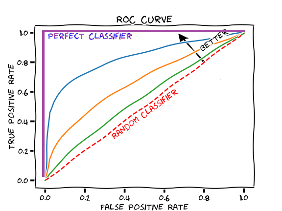
4. AUROC

ROC (Receiver Operating Characteristic) is a plot used to see the quality of the model in many cases of classification problem. The X-axis of ROC curve is False Positive Rate, and the Y-axis of the curve is True Positive Rate. It is created by various thresholds.

False Positive Rate: $\frac{FP}{FP + TN} = 1 - TNR = 1 - Specificity$

True Positive Rate, also Recall, and Sensitivity: $\frac{TP}{TP + FN}$

Therefore, sensitivty and specificity or ROC curve deal with the each two columns of confusion matrix. We can see the overall accuracy by various thresholds with the metrics for both positive and negative values.

The trade-off between Sensitivity and Specificty or ROC curve is quite similar with the trade-off between Precision and Recall as above example shows.

When threshold is 0.1, the Sensitivity is 0.95, and the Specificity is 0.3467, then the FPR will be $1-0.3467 = 0.6533$.

Threshold is 0.1 :

• Sensitivity = 0.95
• Specificity = 0.3467
• FPR = $1-0.3467 = 0.6533$

Threshold is 0.3 :

• Sensitivity = 0.7625
• Specificity = 0.7400
• FPR = $1-0.7400 = 0.26$

Threshold is 0.5 :

• Sensitivity = 0.6125
• Specificity = 0.8667
• FPR = $1-0.8667 = 0.1333$

Threshold is 0.7 :

• Sensitivity = 0.4
• Specificity = 0.9533
• FPR = $1-0.9533 = 0.0467$

In this scenario, we also would think that when the threshold is 0.3 is the optimal cutoff because they seem the optimal values for both. However, we can see the overall quality of the classifier with the AUC values.

AUC (Area Under Curve) is the area under the ROC curve. The greater the AUC value is, the better classifier we get.

Below is the implementation of my own functions for developing all of the above metrics, such as Precision and Recall, Sensitivity and Specificity, ROC curves, and AUC values.

1
2
3
4
5
6
7
8
9
10
11
12
13
14
15
16
17
18
19
20
21
22
23
24
25
26
27
28
29
30
31
32
33
34
35
36
37
38
39
40
41
42
43
44
45
46
47
48
49
50
51
52
53
54
55
56
57
58
59
60
61
62
63
64
65
66
67
68
69
70
71
72
73
74
75
76
77
78
79
80
81
82
83
84
85
86
87
88
89
90
91
92
93
94
95
96
97
98
99
100
101
102
103
104
105
106
107
108
109
110
111
112
113
114
115
116

#This function creates a dataframe that has TP, TN, FP, and FN values
#This function should have same levels for the both target and pred variable
tptnfpfn <- function(x,y){
  tap <- tapply(x,x,length)
  f.names <- tap[1] %>% names
  
  if(tap[1] > tap[2]){
    target <- ifelse(x == f.names, 0, 1)
    pred <- ifelse(y == f.names, 0, 1)
  }
  if(tap[2] > tap[1]){
    target <- ifelse(x == f.names, 1, 0)
    pred <- ifelse(y == f.names, 1, 0)
  }
  
  #target <- x
  #pred <- y
  
  dat <- data.frame(target, pred)
  
  TP <- length(which(dat$target == 1 & dat$pred == 1))
  FP <- length(which(dat$target == 0 & dat$pred == 1))
  TN <- length(which(dat$target == 0 & dat$pred == 0))
  FN <- length(which(dat$target == 1 & dat$pred == 0))
  
  new.dat <- data.frame(TP,FP,TN,FN)
  return(new.dat)
}



#Precision = TP / (TP + FP) <- the denominator is total predicted positive values
precision <- function(tp.dat){
  precision <- tp.dat$TP / (tp.dat$TP + tp.dat$FP)
  return(precision)
}


#Recall = sensitivity = TP / (TP + FN) <- the denominator is total actual positive values 

recall <- function(tp.dat){
  recall <- tp.dat$TP / (tp.dat$TP + tp.dat$FN)
  return(recall)
}

#Sensitivity = Recall

#Specificity = TN / (TN + FP) <- the denominator is total actual negative values
spec <- function(tp.dat){
  specificity <- tp.dat$TN / (tp.dat$TN + tp.dat$FP)
  return(specificity)
}


#ROC = TPR vs FPR = Recall vs 1-TNR = TP/(TP+FN) vs FP/(FP+TN)
roc.func <- function(target,pred){
  dummy <- data.frame(TPR = rep(0, length(target)), 
                      FPR = rep(0, length(target)), 
                      Spec = rep(0,length(target)),
                      Precision = rep(0, length(target)),
                      f1score = rep(0, length(target)))
  
  tap <- tapply(target,target,length)
  if(tap[1] > tap[2]){
    f.name <- levels(as.factor(target))[2]
    s.name <- levels(as.factor(target))[1]
  }
  if(tap[2] > tap[1]){
    f.name <- levels(as.factor(target))[1]
    s.name <- levels(as.factor(target))[2]
  }
  
  for(i in 1:length(target)){
    #splitting the probabilities by cutoff with same levels
    pred.cutoff <- ifelse(pred >= sort(pred)[i], f.name, s.name)
    
    tptn <- tptnfpfn(target,pred.cutoff)
    
    dummy$cutoff[i] <- sort(pred)[i]
    dummy$TPR[i] <- recall(tptn)
    dummy$FPR[i] <- tptn$FP / (tptn$FP + tptn$TN)
    dummy$Spec[i] <- spec(tptn)
    dummy$Precision[i] <- precision(tptn)
    dummy$f1score[i] <- f1.score(tptn)
  }
  
  #dummy$TPR <- ifelse(dummy$TPR == "NaN", 0, dummy$TPR)
  #dummy$FPR <- ifelse(dummy$FPR == "NaN", 0, dummy$FPR)
  return(dummy)
}


#This auc function is from below link. 
#Refer to 
#https://mbq.me/blog/augh-roc/
#a little changes is applied into the codes from above link
#This is using the test statistic from "Mann-Whitney-Wilcoxon test"
#Further link:
#https://en.wikipedia.org/wiki/Mann%E2%80%93Whitney_U_test#Area-under-curve_(AUC)_statistic_for_ROC_curves
auc.func <- function(target, pred){
  tap <- tapply(target, target, length)
  f.name <- tap[1] %>% names
  
  if(tap[1] > tap[2]){
    target1 <- ifelse(target == f.name, TRUE, FALSE)
  }
  if(tap[2] > tap[1]){
    target1 <- ifelse(target == f.name, TRUE, FALSE)
  }
  
  n1 <- sum(!target1)
  n2 <- sum(target1)
  U <- sum(rank(pred)[!target1]) - n1 * (n1 + 1) / 2
  
  return(1 - U / (n1*n2))
}

Below is the results by built-in syntax in R with “ROCR” package

Below is the results by the created functions as above.

Full implementation will be here

Reference:
Precision and Recall
Receiver Operating Characteristic
Type 1 and Type 2 Error
AUC Meets the Wilcoxon-Mann-Whitney U-Statistic