2019-09-15

ML / Gaussian Process

12 minutes read (About 1840 words)

GaussianProcess

Introduction to Gaussian Process

In this post, I will discuss about Gaussian Process, which employs Gaussian distribution (also often called normal distribution that plays an important role in statistics. The previous posts, such as CLT, Cholesky Decomposition, and Schur Complement, are posted because they are needed to understand the Gaussian Process.

Before I start with Gaussian Process, some important properties of Gaussian Distribution will be addressed.

$\large{Gaussian}$ $\large{ Distribution}$

If we have random vector $X$ following Gaussian Distribution, then we have

$$X = \begin{bmatrix} X_1 \\ X_2 \\ … \\ X_n \end{bmatrix} \sim \mathcal{N}(\mu, \Sigma)$$

where $\Sigma = Cov(X_i, X_j) = E[(X_i - \mu_i)(X_j - \mu_j)^{T}]$

Now, Suppose we have two vectors, $X$ and $Y$ that are subsets of a random variable, Z, with the following;

$$P_Z = P_{X,Y} = \begin{bmatrix} X \\ Y \end{bmatrix} \sim \mathcal{N}(\mu, \Sigma) = \mathcal{N}(\begin{bmatrix} \mu_X \\ \mu_Y \end{bmatrix}, \begin{bmatrix} \Sigma_{XX} & \Sigma_{XY} \\ \Sigma_{YX} & \Sigma_{YY} \end{bmatrix})$$

Then, the following properties holds;

1. Normalization

The density function will be

$$\int_{Z} p(Z;\mu,\Sigma) dz = 1$$

where $Z = \begin{bmatrix} X \\ Y \end{bmatrix}$

2. Marginalization

The maginal densities will be

$$p(X) = \int_{Y} p(X,Y; \mu, \Sigma) dy \\ p(Y) = \int_{X} p(X,Y; \mu, \Sigma) dx$$

which are Gaussian, therefore

$$X \sim \mathcal{N}(\mu_X, \Sigma_{XX}) \\ Y \sim \mathcal{N}(\mu_Y, \Sigma_{YY})$$

3. Conditioning

The conditional densities will also be Gaussian, and the conditional expected value and covariance are calculated with the properties of Schur Complement as the following.

Refer to the wiki, Schur Complement.

The conditional expectation and covariance of X given Y is the Schur Complement of C in $\Sigma$ where if $\Sigma$ is defined as

$$\Sigma = \begin{bmatrix} A & B \\ B^{T} & C \end{bmatrix}$$

$$Cov(X|Y) = A-BC^{-1}B^{T} \\ E(X|Y) = E(X) + BC^{-1}(Y-E(Y))$$

Hence, the conditional covariance of X given Y will be

$$P_{X,Y} = \mathcal{N}(\begin{bmatrix} \mu_X \\ \mu_Y \end{bmatrix}, \begin{bmatrix} \Sigma_{XX} & \Sigma_{XY} \\ \Sigma_{YX} & \Sigma_{YY} \end{bmatrix})$$

$$X | Y \sim \mathcal{N}(\mu_X + \Sigma_{XY}\Sigma_{YY}^{-1}(Y-\mu_Y), \Sigma_{XX} - \Sigma_{XY}\Sigma_{YY}^{-1}\Sigma_{YX}) \\
Y | X \sim \mathcal{N}(\mu_Y + \Sigma_{YX}\Sigma_{XX}^{-1}(X-\mu_X), \Sigma_{YY} - \Sigma_{YX}\Sigma_{XX}^{-1}\Sigma_{XY})$$

4. Summation

The sum of independent Gaussian random variables is also Gaussian;

Let $y \sim \mathcal{N}(\mu, \Sigma)$ and $z \sim \mathcal{N}(\mu’,\Sigma’)$

Then,

$$y + z \sim \mathcal{N}(\mu + \mu’, \Sigma+\Sigma’)$$

We see some of important properties of Gaussian distribution.

Now, let’s change our focus to linear regression problem.

Typical linear regression equation is defined as,

$$y = ax + b$$

Or,

$$y = \beta_0 + \beta_1X_1 + … + \beta_pX_p + \epsilon$$

And, it can be expressed by

$$y = f(x) + \epsilon$$

where $f(x) = \beta_0 + \beta_1X_1 + … + \beta_pX_p$.

Here, an important assumption of linear regression is that the error term, $\epsilon$ is normally distributed with mean zero.

If we consider repeated sampling from our population, for large sample sizes, the distribution of the ordinary least squared estimates of the regression coefficients follow a normal distribution by the Central Limit Theorem.

Refer to the previous post, Central Limit Theorem

Therefore, the $\epsilon$ follows Gaussian Distribution.

We might then think about what if our $f(x)$ follows Gaussian distribution.

Then, in the above equation, $y = f(x) + \epsilon$ will follow Gaussian distribution by the property that the sum of two independent Gaussian distribution is Gaussian distribution.

Here is the start of the Gaussian Process.

$\large{Gaussian}$ $\large{ Process}$

A Gaussian Process is one of stochastic process that is a collection of random variables, ${f(x) : x \in \mathcal{X}}$, indexed by elements from some set $\mathcal{X}$, known as the index set, and GP is such stochastic process that any finite subcollection of random variables has a multivariate Gaussian distribution.

Here, we assume the $f(x)$ follows Gaussian distribution with some $\mu$ and $\Sigma$.

The $\mu$ and $\Sigma$ are called as “mean function” and “covariance function” with the notation,

$$f(.) \sim \mathcal{GP}(m(.), k(.,.))$$

where $k(.,.)$ is covariance function and a kernel function.

Hence, we have the equation,

$$y^{i} = f(x^{i}) + \epsilon^{i}$$

where the error term (“noise”), $\epsilon^{i}$ with independent $\mathcal{N}(0, \sigma^2)$ distribution.

We assume the prior distribution over the function $f(.)$ with mean zero Gaussian;

$$f(.) \sim \mathcal{GP}(0, k(.,.))$$

for some valid kernel function $k(.,.)$.

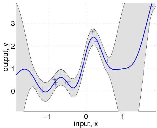
Now, we can convert the $\mathcal{GP}$ prior $f(.)$ into a $\mathcal{GP}$ posterior function after having some data to make predictions $f_p$.

Then, the two functions for the training ($f(.)$) and test ($f_p(.)$), will follows

$$\begin{bmatrix} f \\ f_p \end{bmatrix}|X,X_p \sim \mathcal{N}\big(0, \begin{bmatrix} K(X,X) & K(X, X_p) \\ K(X_p, X) & K(X_p, X_p) \end{bmatrix}\big)$$

Now, with $\epsilon$ and $\epsilon_p$,

$$\begin{bmatrix} \epsilon \\ \epsilon_p\end{bmatrix} \sim \mathcal{N}(0,\begin{bmatrix} \sigma^2I & 0 \\ 0^{T} & \sigma^2I\end{bmatrix})$$

As mentioned above, the sum of two independent Gaussian distribution is also Gaussian, then eventually we have,

$$\begin{bmatrix} y \\ y_p \end{bmatrix} | X, X_p = \begin{bmatrix} f \\ f_p \end{bmatrix} + \begin{bmatrix} \epsilon \\ \epsilon_p\end{bmatrix} \sim \mathcal{N}(0, \begin{bmatrix} K(X,X) + \sigma^2I & K(X,X_p) \\ K(X_p, X) & K(X_p,X_p)+\sigma^2I \end{bmatrix})$$

Here, we generate the prior distributions, which are multivariate normal distributions, with standard multivariate normal distribution and the Cholesky factor as the following.

Refer to my previous post for Cholesky Decomposition, Cholesky Decomposition post.

1) Compute covariance function, $\Sigma$, and Cholesky Decomposition for $\Sigma = LL^{T}$

2) Generate standard multivariate normal distribution, $u \sim \mathcal{N}(0,1)$

3) Compute $x = \mu + Lu$, then $x$ will the prior distribution for $\mathcal{GP}$.

Back to our prediction with GP, we have

$$y_p|y,X,X_p \sim \mathcal{N}(\mu_p, \Sigma_p)$$

by the rules for conditioning Gaussians as we have done above.

Then, we have

$$\mu_p = K(X_p, X)K((X,X)+\sigma^2I)^{-1}y \\ \Sigma_p = K(X_p, X_p) + \sigma^2I - K(X_p,X)(K(X,X)+\sigma^2I)^{-1}K(X,X_p)$$

Here, the conditional mean and covariance function are calculated by the Schur Complement as shown above, and since the mean is zero vector, the mean function is defined as the above.

Conditional expectation and covariance with Schur Complement again,

$$\Sigma = \begin{bmatrix} A & B \\ B^{T} & C \end{bmatrix}$$

$$Cov(X|Y) = A-BC^{-1}B^{T} \\ E(X|Y) = E(X) + BC^{-1}(Y-E(Y))$$

Here, the $E(X)$ and $E(Y) = 0$ for $\mathcal{GP}$, thus we have just $BC^{-1}Y$ term, which is $\mu_p = K(X_p, X)K((X,X)+\sigma^2I)^{-1}y$

Kernel Function, $K(.,.)$?

Commonly used kernel function for $\mathcal{GP}$ is squared exponential kernel function, which is often called Gaussian kernel.

It’s defined as,

$$K(X,X_p) = exp(-\frac{1}{2\nu} ||X-X_p||^2) = exp(-\frac{1}{2\nu} (X-X_p)^{T}(X-X_p))$$

where the $\nu$ is the free parameter for bandwidth of the function smoothness.

Here is the implementation of Gaussian Process in R.

xcor <- seq(-5,4.9,by=0.1) #index or coordinate for our data

#Kernel Function (Squared exponential kernel function or Gaussian kernel function)
GP.kernel <- function(x1,x2,l){
  mat <- matrix(rep(0, length(x1)*length(x2)), nrow=length(x1))
  for (i in 1:length(x1)) {
    for (j in 1:length(x2)) {
      mat[i,j] <- (x1[i]-x2[j])^2
    }
  }
  kern <- exp(-(0.5*mat)/l) #l is free parameter that can be seen as bandwidth
  return(kern)
}


#Zero-mean and covariance function by the squared exponential kernel function with the index to create prior distribution
mu <- rep(0,length(xcor))
cov <- GP.kernel(xcor,xcor,1) #nu is 1


#3 prior distributions
dat <- data.frame(x=xcor, first=mvrnorm(1,mu,cov), sec=mvrnorm(1,mu,cov), thi=mvrnorm(1,mu,cov))
#mvrnorm function is same with the using of Cholesky factor of the covariance function multiplied by the standard multivariate normal distribution added mu



#graph for the 3 priors
dat %>% ggplot() + 
  geom_line(aes(x=xcor,y=first, colour="red")) + 
  geom_line(aes(x=xcor,y=sec, colour="blue")) +
  geom_line(aes(x=xcor,y=thi, colour="green"))

#Assume we have a data

#5 elements
f <- data.frame(x=c(-4,-3,-1,0,2),
                y=c(-2,0,1,2,-1))
x <- f$x
k.xx <- GP.kernel(x,x,1)
k.xxs <- GP.kernel(x,xcor,1)
k.xsxs <- GP.kernel(xcor,xcor,1)


f.star.bar <- t(k.xxs)%*%solve(k.xx)%*%f$y #mean function
cov.f.star <- k.xsxs - t(k.xxs)%*%solve(k.xx)%*%k.xxs #covariance function

#posterior distribution
dat1 <- data.frame(x=xcor, 
                  first=mvrnorm(1,f.star.bar,cov.f.star), 
                  sec=mvrnorm(1,f.star.bar,cov.f.star), 
                  thi=mvrnorm(1,f.star.bar,cov.f.star))

#graph for 3 posterior distribution when nu is 1
dat1 %>% ggplot() + 
  geom_line(aes(x=xcor,y=first, colour="red")) + 
  geom_line(aes(x=xcor,y=sec, colour="blue")) +
  geom_line(aes(x=xcor,y=thi, colour="green")) +
  geom_line(aes(x=xcor,y=f.star.bar),colour="black")+
  geom_errorbar(data=f, aes(x=x, y=NULL, ymin=y-2*0.1, ymax=y+2*0.1),width=0.2)+
  geom_point(data=f,aes(x=x,y=y)) +
  ggtitle("Posterior from Prior x likelihood/evidence (given x,x*,y)")


mu <- rep(0,length(xcor))
cov <- GP.kernel(xcor,xcor,0.1) #nu is 0.1

dat <- data.frame(x=xcor, first=mvrnorm(1,mu,cov), sec=mvrnorm(1,mu,cov), thi=mvrnorm(1,mu,cov))

dat %>% ggplot() + 
  geom_line(aes(x=xcor,y=first, colour="red")) + 
  geom_line(aes(x=xcor,y=sec, colour="blue")) +
  geom_line(aes(x=xcor,y=thi, colour="green")) +
  ggtitle("When sigma is 0.1")


mu <- rep(0,length(xcor))
cov <- GP.kernel(xcor,xcor,10) #nu is 10


dat <- data.frame(x=xcor, first=mvrnorm(1,mu,cov), sec=mvrnorm(1,mu,cov), thi=mvrnorm(1,mu,cov))

dat %>% ggplot() + 
  geom_line(aes(x=xcor,y=first, colour="red")) + 
  geom_line(aes(x=xcor,y=sec, colour="blue")) +
  geom_line(aes(x=xcor,y=thi, colour="green")) +
  ggtitle("When sigma is 10")